1. Introduction to Python With ANSWERS

Table of Contents

• 1. Introduction to Python With ANSWERS

  • 1.1 Getting Started

    • 1.1.1 Comments and print function

    • 1.1.2 Variables, Values and Data types

    • 1.1.3 Arithmetic

    • 1.1.4 Assignment Operators

    • 1.1.5 Logical Operators

    • 1.1.6 Comparison Operators and if

    • 1.1.7 Summary

  • 1.2 Text and looping

    • 1.2.1 len

    • 1.2.2 for … in … and enumerate

    • 1.2.3 slice

    • 1.2.4 replace

    • 1.2.5 find

    • 1.2.5 split and splitlines

    • 1.2.6 Summary

  • 1.3. Groups of things

    • 1.3.1 tuple

    • 1.3.2 list

    • 1.3.3 np.array

    • 1.3.4 dict

    • 1.3.5 Summary

Python is a popular general purpose, free language. As opposed to other systems that are focused towards a particular task (e.g. R for statistics), Python has a strong following on the web, on systems operations and in data analysis. For scientific computing, a large number of useful add-ons (“libraries”) are available to help you analyse and process data. This is an invaluable resource.

In addition to being free, Python is also very portable, and easy to pick up.

The aim of this Chapter is to introduce you to some of the fundamental concepts in Python. Mainly, this is based around fundamental data types in Python (int, float, str, bool etc.) and ways to group them (tuple, list, array, string and dict).

Although some of the examples we use are very simple to explain a concept, the more developed ones should be directly applicable to the sort of programming you are likely to need to do.

Further, a more advanced section of the chapter is available, that goes into some more detail and complkications. This too has a set of exercises with worked examples.

In this session, you will be introduced to some of the basic concepts in Python.

The session should last 4 hours (one week).

1.1 Getting Started

1.1.1 Comments and print function

Comments are statements ignored by the language interpreter.

Any text after a # in a code block is a comment.

You can ‘run’ the code in a code block using the ‘run’ widget (above) or hitting the keys (‘typing’) and at the same time.

E1.1.1 Exercise

• Try running the code block below
• Explain what happened (‘what the computer did’)

# Hello world

ANSWER

Nothing ‘apparently’ happened, but really, the code block was interpreted as a set of Python commands and executed. As there is only a comment, there was no output.

You can also use text blocks (contained in quotes) to contain comments, but note that if it is the last statement in the code, the text block may be printed out to the terminal.

# single line text
'hello world is not printed'

# multi-line text
'''
Hello
world
is printed
'''

'nHello nworldnis printedn'

E1.1.2 Exercise

• Copy the text from above in the window below
• Then put a new text block at the end and note down what happens
• What does the \n mean/do?

# do the exercise here
# ANSWER

# single line text
'hello world is not printed'

# multi-line text
'''
Hello
world
is printed
'''

'''
Another text block
'''

'nAnother text blockn'

ANSWER

The last output is printed. In this case, it is the string '\nAnother text block\n'.

The \n is a newline character. It setrs the text cursor to the start of a new line.

To print some statement (by default, to the screen you are using), use the print method:

print('hello world')

hello world

print('hello','world')

hello world

In Python 3.X, print is a function with the argument(s) (here, the string you want printed) enclosed in the function’s (round) brackets.

E1.1.3 Exercise

• Copy the print statement from above code block.
• Change the words in the quotes and print them out.
• Add some comments to the code block explaining what you have done and seen.

# do the exercise here
# ANSWER


'''
The print statement below sends text to the output channel (the 'screen' as it were).
In this case, it prints the string 'good', followed by a space, then the string 'morning'
'''
print('good','morning')

good morning

1.1.2 Variables, Values and Data types

The idea of variables is fundamental to any programming. You can think of this as the name of something, so it is a way of allowing us to refer to some object in the language.

What the variable is set to is called its value.

So let’s start with a variable we will call (declare to be) x.

We will give a value of the string 'one' to this variable:

x = 'one'

print(x)

one

E1.1.4 Exercise

• set the a variable called x to some different string (e.g. ‘hello world’)
• print the value of the variable x
• Try this again, putting some ‘newlines’ (\n) in the string

# do the exercise here
# ANSWER

x = 'hello world'

print(x)
'''
Note the space before the final
hello world, as there is a comma
between '\n' and x
'''
print(x,'\n',x)

hello world
hello world
 hello world

# Now we set x to the value 1

x = 1

print(x,'is type',type(x))

1 is type <class 'int'>

In a computing language, the sort of thing the variable can be set to is called its data type.

In python, we can access this with the method type() as in the example above.

In the example above, the datatype is an integer number (e.g. 1, 2, 3, 4).

In ‘natural language’, we might read the example above as ‘x is one’.

E1.1.5 Exercise

• set the a variable called x to the integer 5
• print the value and type of the variable x
• change the data type used for x to something else (e.g. a string)

# do the exercise here
# ANSWER

x = 5
'''
We use the methods type() and str() here
'''
print(x,type(x),str(x))

5 <class 'int'> 5

Setting x = 1 is different to:

x = 'one'

because here we have set value of the variable x to a string (i.e. some text).

A string is enclosed in quotes, e.g. "one" or 'one', or even "'one'" or '"one"'.

print ("one")
print ('one')
print ("'one'")
print ('"one"')

one
one
'one'
"one"

E1.1.6 Exercise

• create a variable name containing your name, as a string.
• using this variable and the print function, print out a statement such as my name is Fred (if your name were Fred)

# do the exercise here
# ANSWER

name = 'Professor Philip Lewis'
print('My name is',name)

My name is Professor Philip Lewis

Setting x = 1 or x = 'one' is different to:

x = 1.0

because here we have set value of the variable x to a floating point number (these are treated and stored differently to integers in computing).

This in turn is different to:

x = True

where True is a logical or boolean datatype (something is True or False).

E1.1.7 Exercise

• in the code block below, create a variable called my_var and set it to some value (your choice of value, but be clear about the data type you intend)
• print the value of the variable to the screen, along with the data type.

# do the exercise here
# ANSWER

# set to integer
my_var = 100
print(my_var,type(my_var))

100 <class 'int'>

We have so far seen four datatypes:

• integer (int): 32 bits long on most machines
• (double-precision) floating point (float): (64 bits long)
• Boolean (bool)
• string (str)

but we will come across more (and even create our own!) as we go through the course.

In each of these cases above, we have used the variable x to contain these different data types.

As we saw above, if you want to know what the data type of a variable is, you can use the method type()

print (type(1));
print (type(1.0));
print (type('one'));
print (type(True));

<class 'int'>
<class 'float'>
<class 'str'>
<class 'bool'>

You can explicitly convert between data types, e.g.:

print ('int(1.1) = ',int(1.1))
print ('float(1) = ',float(1))
print ('str(1) = ',str(1))
print ('bool(1) = ',bool(1))

int(1.1) =  1
float(1) =  1.0
str(1) =  1
bool(1) =  True

but only when it makes sense:

print ("converting the string '1' to an integer makes sense:",int('1'))

converting the string '1' to an integer makes sense: 1

print ("converting the string 'one' to an integer doesn't:",int('one'))

---------------------------------------------------------------------------

ValueError                                Traceback (most recent call last)

<ipython-input-23-11bdc0c0e878> in <module>
----> 1 print ("converting the string 'one' to an integer doesn't:",int('one'))


ValueError: invalid literal for int() with base 10: 'one'

When you get an error (such as above), you will need to learn to read the error message to work out what you did wrong.

E1.1.8 Exercise

• why did the statement above not work?
• type some other data conversions below that do work.

# do the exercise here
# ANSWER

print(str(1),str('1 2 3'))
print(int('1'))

1 1 2 3
1

We tried to convert a string (‘one’) to an integer, that doesn’t make sense. It is ok e.g. for int('1') though.

1.1.3 Arithmetic

Often we will want to do some arithmetic with numbers in a program, and we use the ‘normal’ (derived from C) operators for this.

Note the way this works for integers and floating point representations.

'''
    Some examples of arithmetic operations in Python

    Note how, if we mix float and int, the result is raised to float
    (as the more general form)
'''

print (10 + 100)     # int addition
print (10. - 100)    # float subtraction
print (1./2.)        # float division
print (1/2)          # int division
print (10.*20.)      # float multiplication
print (2 ** 3.)      # float exponent

print (65%2)         # int remainder
print (65//2)        # floor operation

110
-90.0
0.5
0.5
200.0
8.0
1
32

E1.1.9 Exercise

• change the numbers in the examples above to make sure you understand these basic operations.
• try combining operations and use brackets () to check that that works as expected.
• see what happens when you add (i.e. use +) strings together

# do the exercise here
# ANSWER

print (1 + 10)     # int addition
print (1. - 10)    # float subtraction
print (3./2.)        # float division
print (3/2)          # int division
print (1.*2.)      # float multiplication
print (2 ** 8.)      # float exponent

print (129%2)         # int remainder
print (129//2)        # floor operation

11
-9.0
1.5
1.5
2.0
256.0
1
64

Most of these are obvious. The integer division in this case returns a float, which is a change from Pythjon 2.

The remainder and floor terms mean that 129 = 64 * 2 + 1, i.e. 129 = floor * 2 + remainder

1.1.4 Assignment Operators

'''
    Assignment operators

    x = 3   assigns the value 3 to the variable x
    x += 2  adds 2 onto the value of x
            so is the same as x = x + 2
            similarly /=, *=, -=
    x %= 2  is the same as x = x % 2
    x **= 2 is the same as x = x ** 2
    x //= 2 is the same as x = x // 2

    A 'magic' trick
    ===============

    based on
    https://www.wikihow.com/Read-Someone%27s-Mind-With-Math-(Math-Trick)

    whatever you put as myNumber, the answer is 42

    Try this with integers or floating point numbers ...
'''

# pick a number
myNumber = 34.67

x = myNumber

x *= 2

x *= 5

x /= myNumber

x -= 7

x += 39

# The answer will always be 42
print(x)

42.0

E1.1.10 Exercise

• change the number assigned to myNumber and check if 42 is still returned
• copy and edit the code to print the value of x each time you change it, and add comments explaining what is happening for each line of code. This should allow you to follow more carefully what has happened with the arithmetic and also to simplify the code (use fewer statements to achieve the same thing).

# do the exercise here
# ANSWER

myNumber = 27.6
x = myNumber
print(x)
x *= 2
print(x)
x *= 5
print(x)
x /= myNumber
print(x)
x -= 7
print(x)
x += 39
# The answer will always be 42
print(x)

27.6
55.2
276.0
10.0
3.0
42.0

# do the exercise here
# ANSWER ... not so magic after all

myNumber = 27.6

x = 10
print(x)
x += 32
# The answer will always be 42
print(x)

10
42

1.1.5 Logical Operators

Logical operators combine boolean variables. Recall from above:

print (type(True),type(False));

<class 'bool'> <class 'bool'>

The three main logical operators you will use are:

not, and, or

The impact of the not opeartor should be straightforward to understand, though we can first write it in a ‘truth table’:

A	not A
T	F
F	T

print('not True is',not True)
print('not False is',not False)

not True is False
not False is True

E1.1.11 Exercise:

• write a statement to set a variable x to True and print the value of x and not x
• what does not not x give? Make sure you understand why

# do the exercise here
# ANSWER

x = True
print(x)
print(not x)
print(not not x)

True
False
True

not not cancels out.

The operators and and or should also be quite straightforward to understand: they have the same meaning as in normal english. Note that or is ‘inclusive’ (so, read A or B as ‘either A or B or both of them’).

print ('True and True is',True and True)
print ('True and False is',True and False)
print ('False and True is',False and True)
print ('False and False is',False and False)

True and True is True
True and False is False
False and True is False
False and False is False

So, A and B is True, if and only if both A is True and B is True. Otherwise, it is False

We can represent this in a ‘truth table’:

A	B	A and B
T	T	T
T	F	F
F	T	F
F	F	F

E1.1.12 Exercise:

• draw a truth table on some paper, label the columns A, B and A and B and fill in the columns A and B as above
• without looking at the example above, write the value of A and B in the third column.
• draw another truth table on some paper, label the columns A, B and A and B and fill in the columns A and B as above
• write the value of A or B in the third column.

If you are unsure, test the response using code, below.

# do the testing here e.g.
print (True or False)

True

ANSWER

E1.1.13 Exercise

• Copy the following truth table onto paper and fill in the final column:

A	B	C	((A and B) or C)
T	T	T
T	T	F
T	F	T
T	F	F
F	T	T
F	T	F
F	F	T
F	F	F

• Try some other compound statements

If you are unsure, or to check your answers, test the response using code, below.

# do the testing here e.g.
print ((True and False) or True)

True

ANSWER

Do it one statement at a time:

A	B	C	A and B	(A and B) or C
T	T	T	T	T
T	T	F	T	T
T	F	T	F	T
T	F	F	F	F
F	T	T	F	T
F	T	F	F	F
F	F	T	F	T
F	F	F	F	F

1.1.6 Comparison Operators and if

A comparison operator ‘compares’ two terms (e.g. variables) and returns a boolean data type (True or False).

For example, to see if the value of some variable a is ‘the same value as’ (‘equivalent to’) the value of some variable b, we use the equivalence operator (==). To test for non equivalence, we use the not equivalent operator != (read the ! as ‘not’):

a = 100
b = 10

# Note the use of \n and \t in here
#
print ('a is',a,'and\nb is',b,'\n')
print ('\ta is equivalent to b?',a == b)

a is 100 and
b is 10

    a is equivalent to b? False

E1.1.14 Exercise

• copy the code above and change the values (or type) of the variables a and b to test their equivalence.
• what does the \t in the print statement do?
• add a print statement to your code that tests for ‘non equivalence’
• write some code to see if (a or b) is equivalent to (b or a) or not

# do the exercise here
# ANSWER

# for logical operators
a = True
b = False

# Note the use of \n and \t in here
#
print ('a is',a,'and\nb is',b,'\n')
print ('\ta is equivalent to b?',a == b)
print ('\ta is not equivalent to b?',a != b)
print ('\t(a or b) == (b or a)?',(a or b) == (b or a))

# for other comparisons ... the or works differently
a = 10
b = 20

# Note the use of \n and \t in here
#
print ('a is',a,'and\nb is',b,'\n')
print ('\ta is equivalent to b?',a == b)
print ('\ta is not equivalent to b?',a != b)
print ('\t(a or b) == (b or a)?',(a or b) == (b or a))

# this just sets to a and b respectively, since True
print((a or b),(b or a))

a is True and
b is False

    a is equivalent to b? False
    a is not equivalent to b? True
    (a or b) == (b or a)? True
a is 10 and
b is 20

    a is equivalent to b? False
    a is not equivalent to b? True
    (a or b) == (b or a)? False
10 20

A full set of comparison operators is:

symbol meaning

== is equivalent to != is not equivalent to > greater than >= greater than or equal to < less than <= less than or equal to ====== ===============================================================================

so that, for example:

# Comparison examples

# is one plus one list identical to two list?
print ([1 + 1] is [2])

# is one plus one list equal to two list?
print ([1 + 1] == [2])

# is one less than or equal to 0.999?
print (1 <= 0.999)

# is one plus one not equal to two?
print (1 + 1 != 2)

# note the use of single quotes inside a double quoted string here
# is 'more' greater than 'less'?
print ("more" > "less")

# "is 100 less than 2?"
print (100 < 2)

False
True
False
False
True
False

Aside on string comparisons

In the case of string comparisons, the ASCII codes of the string characters are compared. So for example the statement “more” > “less” returns True.

Here, the comparison is effectively

m > l

Since m comes after l in the alphabet, the ASCII code for m (109) is greater than the ASCII code for l (108) (see http://www.asciitable.com) so

109 > 108

returns True. Note that ASCII capital letters come before the lower case letters.

In practice, we mainly avoid string comparisons (other than to confirm equivalence). So there is little direct use of string comparisons other than ==. It is useful to know how this works however, in case it crops up or happens ‘by accident’. It is also worth understanding what ASCII codes are.

Conditional test

One common use of comparisons is for program control, using an if statement:

if condition1 is True:
    doit1()
elif condition2 is True:
    doit2()
else:
    doit3()

where is compares identity. This allows us to run blocks of code (e.g. the method doit1()) only under a particular condition (or set of conditions).

In Python, the statement(s) we run on condition (here doit1() etc.) are indented.

The indent can be one or more spaces or a <tab> character, the choice is up to the programmer. However, it must be consistent.

test = [1+1]
print('test is {}'.format(test))

# initialise retval
retval = None

# conduct some tests, and set the
# variable retval to True if we pass
# any test

if test is [2]:
    retval = True
    print('passed test 1: "if test is [2]"')
elif test == [2]:
    retval = True
    print('passed test 2: "if test == [2]"')
else:
    retval = False
    print('failed both tests')

print('retval is',retval)

test is [2]
passed test 2: "if test == [2]"
retval is True

E1.1.15 Exercise

• copy the example above, and change it to use other examples from the ‘Comparison examples’ code block. Change the value of test to get different responses and make notes as to why you get the result you do.
• try out some more complicated conditions, e.g. multipler tests, combined with an and operator.

# do the exercise here
# ANSWER

test = [3 / 2]
print('test is {}'.format(test))

# initialise retval
retval = None

# conduct some tests, and set the
# variable retval to True if we pass
# any test

if test is [1.5]:
    retval = True
    print('passed test 1: "if test is [1.5]"')
elif test == [1]:
    retval = True
    print('passed test 2: "if test == [1]"')
else:
    retval = False
    print('failed both tests')

print('retval is',retval)

test is [1.5]
failed both tests
retval is False

So be careful how you use is. It is not the same as == which only tests for equivalence. is is really a pointer comparison, so are they the same object?

In this section, you have had an introduction to the Python programming language, running in a `jupyter notebook <http://jupyter.org>`__ environment.

You have seen how to write comments in code, how to form print statements and basic concepts of variables, values, and data types. You have seen how to maniputae data with arithmetic and assignment operators, as well as the basics in dealing with logic and tests returning logical values.

1.2 Text and looping

In Python, collections of characters (a, b, 1, …) are called strings. Strings and characters are input by surrounding the relevant text in either double (") or single (') quotes. There are a number of special characters that can be encoded in a string provided they’re “escaped”. For example, some we have come across are:

• \n: the carriage return
• \t: a tabulator

print ("I'm a happy string")
print ('I\'m a happy string') # the apostrophe has been escaped as not to be confused by end of string
print ("\tI'm a happy string")
print ("I'm\na\nhappy\nstring")

I'm a happy string
I'm a happy string
    I'm a happy string
I'm
a
happy
string

We can do a number of things with strings, which are very useful. These so-called string methods are defined on all strings by Python by default, and can be used with every string. For one, we can concatenate strings using the + symbol as we saw above.

1.2.1 len

Gives the length of the string as number of characters:

t = ''
print ('the length of',t,'is',len(t))


s = "Hello" + "there" + "everyone"

print ('the length of',s,'is',len(s))

the length of  is 0
the length of Hellothereeveryone is 18

Exercise E1.2.1

• what does a zero-length string look like?
• The Hello there everyone example above has no spaces between the words. Copy the code to the block below and modify it to have spaces.
• confirm that you get the expected increase in length.

# do exercise here
# ANSWER

zero = ''
s = "Hello" + " " + "there" + " " +  "everyone"
print(s)
print ('the length of',s,'is',len(s))

Hello there everyone
the length of Hello there everyone is 20

1.2.2 for ... in ... and enumerate

Very commonly, we need to iterate or ‘loop’ over some set of items.

The basic stucture for doing this (in Python, and many other languages) is for item in group:, where item is the name of some variable and group is a set of values.

The loop is run so that item takes on the first value in group, then the second, etc.

# for loop
group = [4,3,2,1]

for item in group:
    '''print counter in loop'''
    print(item)

print ('blast off!')

4
3
2
1
blast off!

The group in this example is the list of integer numbers [4,3,2,1]. A list is a group of comma-separated items contained in square brackets [].

In Python, the statement(s) we run whilst looping (here print(item)) are indented.

The indent can be one or more spaces or a <tab> character, the choice is up to the programmer. However, it must be consistent.

Exercise 1.2.1

• generate a list of strings called group with the names of (some of) the items in your pocket or bag (or make some up!)
• set up a for loop to go through and print each item

# do exercise here
# ANSWER

group = ['cat','fish','egg']
for item in group:
    print('I have',item,'in my pocket')

I have cat in my pocket
I have fish in my pocket
I have egg in my pocket

Quite often, we want to keep track of the ‘index’ of the item in the loop (the ‘item number’).

One way to do this would be to use a variable (called count here).

Before we enter the loop, we initialise the value to zero.

# for loop
group = ['hat','dog','keys']

# initialise a variable count
count = 0

for item in group:
    '''print counter in loop'''

    print('item',count,'is',item)

    # add 1 onto count
    count += 1

item 0 is hat
item 1 is dog
item 2 is keys

Exercise 1.2.2

• copy the code above, and check to see if the value of count at the end of the loop is the same as the length of the list. Why should this be so?
• change the code so that the counting starts at 1, rather than 0.

# do exercise here
# ANSWER

# for loop
group = ['hat','dog','keys']

# initialise a variable count
count = 0

for item in group:
    '''print counter in loop'''

    print('item',count,'is',item)

    # add 1 onto count
    count += 1
'''
Expect the same as we have incremented
count once for each item in group, so it
should be the same as the length of the group!
'''
print(count,len(group))

item 0 is hat
item 1 is dog
item 2 is keys
3 3

Since counting in loops is a common task, we can use the built in method enumerate() to achieve the same thing as above. The syntax is then:

# for loop
group = ['hat','dog','keys']

for count,item in enumerate(group):
    '''print counter in loop'''
    print('item',count,'is',item)

item 0 is hat
item 1 is dog
item 2 is keys

Exercise 1.2.3

• copy the code above, and check to see if the value of count at the end of the loop is the same as the length of the list.
• change the code so that the printed count starts at 1, rather than 0.

Hint: how can you make it print count+1 rather than count?

# do exercise here
# ANSWER

# for loop
group = ['hat','dog','keys']

for count,item in enumerate(group):
    '''print counter in loop'''
    print('item',count,'is',item)

'''
In this case, count starts at 0 and takes the
values 0, 1 and 2 as we loop over the 3 items.
'''
print(count,len(group))
'''
print count + 1 !!
'''
print('item',count+1,'is',item)

item 0 is hat
item 1 is dog
item 2 is keys
2 3
item 3 is keys

1.2.3 slice

A string can be thought of as an ordered ‘array’ of characters.

So, for example the string hello can be thought of as a construct containing h then e, l, l, and o.

We can index a string, so that e.g. 'hello'[0] is h, 'hello'[1] is e etc.

We have seen above the idea of the ‘length’ of a string. In this example, the length of the string hello is 5.

string = 'hello'

# length
slen = len(string)
print('length of {} is {}'.format(string,slen))

# select these indices
indices = 0,1,3

# loop over each item in indices
for index in indices:
    print('character {} of {} is {}'.format(index,string,string[index]))

length of hello is 5
character 0 of hello is h
character 1 of hello is e
character 3 of hello is l

Exercise E1.2.4

• copy the code above, and see what happens if you set a value in indices that is the value of length of the string. Why does it respond so?
• make the code robust to this issue, but using an if statement to test if index is in the required range.

# do exercise here
# ANSWER

string = 'hello'

# length
slen = len(string)
print('length of {} is {}'.format(string,slen))

# select these indices
indices = 0,1,3,6

# loop over each item in indices
'''
WE expect a failure as we have
asked for an out of range index
'''

for index in indices:
    print('character {} of {} is {}'.format(index,string,string[index]))

length of hello is 5
character 0 of hello is h
character 1 of hello is e
character 3 of hello is l

---------------------------------------------------------------------------

IndexError                                Traceback (most recent call last)

<ipython-input-68-88baf263801d> in <module>
     18
     19 for index in indices:
---> 20     print('character {} of {} is {}'.format(index,string,string[index]))
     21


IndexError: string index out of range

# do exercise here
# ANSWER

string = 'hello'

# length
slen = len(string)
print('length of {} is {}'.format(string,slen))

# select these indices
indices = 0,1,3,6

# loop over each item in indices
'''
Fix by using condition
'''

for index in indices:
    if index < slen:
        print('character {} of {} is {}'.format(index,string,string[index]))
    else:
        print('index {} beyond the string length {}'.format(index,slen))

length of hello is 5
character 0 of hello is h
character 1 of hello is e
character 3 of hello is l
index 6 beyond the string length 5

We can use the idea of a ‘slice’ to access particular elements within the string.

For a slice, we can specify:

• start index (0 is the first)
• stop index (not including this)
• skip (do every ‘skip’ character)

When specifying this as array access, this is given as, e.g.:

array[start:stop:skip]

• The default start is 0
• The default stop is the length of the array
• The default skip is 1

You can specify a slice with the default values by leaving the terms out:

array[::2]

would give values in the array array from 0 to the end, in steps of 2.

This idea is fundamental to array processing in Python. We will see later that the same mechanism applies to all ordered groups.

s = "Hello World"
print (s,len(s))

start = 0
stop  = 11
skip  = 2
print (s[start:stop:skip])

# use -ve numbers to specify from the end
# use None to take the default value

start = -3
stop  = None
skip  = 1
print (s[start:stop:skip])

Hello World 11
HloWrd
rld

Exercise E1.2.5

The example above allows us to access an individual character(s) of the array.

• copy the example above, and print the string starting from the default start value, up to the default stop value, in steps of 2.
• write code to print out the 4\(^{th}\) letter (character) of the string s.

# do exercise here
# ANSWER

s = "Hello World"

# take the default start by setting to None
start = None
stop  = None
skip  = 2
print (s[start:stop:skip])

# 4th char ... start at 0 remember!
print(s[3])

HloWrd
l

1.2.4 replace

We can replace all occurrences of a string within a string by some other string. We can also replace a string by an empty string, thus in effect removing it:

print ("I'm a very happy string".replace("happy", "unhappy"))

I'm a very unhappy string

Exercise E1.2.6

• copy the statement above, and use the replace method to make it print out "I'm a happy string".

Hint: you want to replace the string very with, effectively, nothing, i.e. a zero-length string.

# do exercise here
# ANSWER

# note that we replace 'very '
print ("I'm a very happy string".replace("very ", ""))

I'm a happy string

1.2.5 find

Quite often, we might want to find a string inside another string, and potentially give the location (as in characters from the start of the string) where this string occurs. We can use the find method, which will return either a -1 if the string isn’t found, or an integer giving the index of where the string starts (for the first time).

print ("I'm a very happy string".find("a"))
print ("I'm a very happy string".find("happy"))

4
11

Let’s use the idea of find() to sort out a messy table of data that we get from a web page.

First, we need to import the package requests to access some information from a URL (from a web page). The data we get will be in html.

The data we will examine is a dataset of ENSO values for each month of the year from January 1950 to present, made available by NOAA/

If you visit you will see the data table we are interested in. So, how do we ‘grab’ this?

The URL points to html code. When you display this in a browser, it is rendered appropriately.

If you access the html directly, you will get the following:

# Web scraping example

import requests

url = "http://www.esrl.noaa.gov/psd/enso/mei/table.html"

# This line will pull the URL data as a string
txt = requests.get(url).text

# show the first 1000 characters (see 'slice' above: this is the same as [None:1000:None])
print(txt[:1000])

<html>
<head><title>MEI timeseries from Dec/Jan 1940/50 up to the present</title></head>
<body>
<pre>
MEI Index (updated: 13 October 2018)

Bimonthly MEI values (in 1/1000 of standard deviations), starting with Dec1949/Jan1950, thru last
month.  More information on the MEI can be found on the <a href="mei.html">MEI homepage</a>.
Missing values are left blank.  Note that values can still change with each monthly update, even
though such changes are typically smaller than +/-0.1.  All values are normalized for each bimonthly
season so that the 44 values from 1950 to 1993 have an average of zero and a standard deviation of "1".
Responses to 'FAQs' can be found below this table:

YEAR    DECJAN  JANFEB  FEBMAR  MARAPR  APRMAY  MAYJUN  JUNJUL  JULAUG  AUGSEP  SEPOCT  OCTNOV  NOVDEC
1950        -1.03   -1.133  -1.283  -1.071  -1.434  -1.412  -1.269  -1.042  -.631   -.406   -1.138  -1.235
1951        -1.049  -1.152  -1.178  -.511   -.374   .288    .679    .818    .726    .768    .726    .504
1952        .433    .138    .071    .224    -.307   -.756   -.305   -.374   .

We notice the presence of html codes in the text string (e.g. <html>, <pre>). There are particular packages for neatly parsing html (scraping information from web pages), one of the most common being BeautifulSoup. This will tend to be more useful if the html is well fomatted, and the data contained in <table> sections, or similar structures. Here, we just have a block of text in the <pre> section.

If we want to just access the dataset here then, we might notice that the data we want to access starts when we see the string YEAR.

We can use find() to discover the index of this in the string:

start = txt.find('YEAR')

print('start of useful data at index {}\n---------------------------------'.format(start))
print(txt[start:start+1000])

start of useful data at index 688
---------------------------------
YEAR    DECJAN  JANFEB  FEBMAR  MARAPR  APRMAY  MAYJUN  JUNJUL  JULAUG  AUGSEP  SEPOCT  OCTNOV  NOVDEC
1950        -1.03   -1.133  -1.283  -1.071  -1.434  -1.412  -1.269  -1.042  -.631   -.406   -1.138  -1.235
1951        -1.049  -1.152  -1.178  -.511   -.374   .288    .679    .818    .726    .768    .726    .504
1952        .433    .138    .071    .224    -.307   -.756   -.305   -.374   .31     .306    -.328   -.098
1953        .044    .401    .277    .687    .756    .191    .382    .209    .483    .124    .099    .351
1954        -.036   -.027   .154    -.616   -1.465  -1.558  -1.355  -1.456  -1.159  -1.32   -1.113  -1.088
1955        -.74    -.669   -1.117  -1.621  -1.653  -2.247  -1.976  -2.05   -1.829  -1.725  -1.813  -1.846
1956        -1.408  -1.275  -1.371  -1.216  -1.304  -1.523  -1.244  -1.118  -1.35   -1.461  -1.014  -.993
1957        -.915   -.348   .108    .383    .813    .73     .926    1.132   1.117   1.114   1.167   1.268
1958        1.473   1.454   1.313   .991    .673    .812    .7      .421    .171    .237    .501    .691
1959        .553    .81     .502    .202    -.025   -.062   -.112   .111    .092    -.038   -.151   -.247
1960        -.287   -.253   -.082   .007    -.322   -.287   -.318   -.25    -.47    -.332   -.308   -.39
1961        -.15    -.235   -.073   .017    -.302   -.185   -.208   -.3     -.3     -.51    -.416   -.60

If we look again at the web page http://www.esrl.noaa.gov/psd/enso/mei/table.html, we might notice that the end of the useful data is delimited by two newlines and the string (1), i.e., as a string \n\n(1). So we should be able to use find() again to get the location of the end of the data (i.e. stop, in the sense of a slice).

Exercise 1.2.6

• use this observation to form a string called data_table, containing all of the useful data (i.e. txt[start:stop]).
• print the string data_table.

# do exercise here
# ANSWER

start = txt.find('YEAR')
end = txt.find('\n\n(1)')

print('start of useful data at index {}\n---------------------------------'.format(start))
data_table = txt[start:end]

print(data_table)

start of useful data at index 688
---------------------------------
YEAR    DECJAN  JANFEB  FEBMAR  MARAPR  APRMAY  MAYJUN  JUNJUL  JULAUG  AUGSEP  SEPOCT  OCTNOV  NOVDEC
1950        -1.03   -1.133  -1.283  -1.071  -1.434  -1.412  -1.269  -1.042  -.631   -.406   -1.138  -1.235
1951        -1.049  -1.152  -1.178  -.511   -.374   .288    .679    .818    .726    .768    .726    .504
1952        .433    .138    .071    .224    -.307   -.756   -.305   -.374   .31     .306    -.328   -.098
1953        .044    .401    .277    .687    .756    .191    .382    .209    .483    .124    .099    .351
1954        -.036   -.027   .154    -.616   -1.465  -1.558  -1.355  -1.456  -1.159  -1.32   -1.113  -1.088
1955        -.74    -.669   -1.117  -1.621  -1.653  -2.247  -1.976  -2.05   -1.829  -1.725  -1.813  -1.846
1956        -1.408  -1.275  -1.371  -1.216  -1.304  -1.523  -1.244  -1.118  -1.35   -1.461  -1.014  -.993
1957        -.915   -.348   .108    .383    .813    .73     .926    1.132   1.117   1.114   1.167   1.268
1958        1.473   1.454   1.313   .991    .673    .812    .7      .421    .171    .237    .501    .691
1959        .553    .81     .502    .202    -.025   -.062   -.112   .111    .092    -.038   -.151   -.247
1960        -.287   -.253   -.082   .007    -.322   -.287   -.318   -.25    -.47    -.332   -.308   -.39
1961        -.15    -.235   -.073   .017    -.302   -.185   -.208   -.3     -.3     -.51    -.416   -.608
1962        -1.065  -.963   -.692   -1.04   -.89    -.87    -.683   -.538   -.56    -.642   -.598   -.482
1963        -.718   -.837   -.675   -.761   -.473   -.144   .404    .59     .734    .848    .866    .765
1964        .878    .481    -.256   -.545   -1.234  -1.15   -1.384  -1.486  -1.309  -1.196  -1.211  -.907
1965        -.536   -.329   -.259   .086    .464    .867    1.367   1.425   1.379   1.25    1.378   1.27
1966        1.307   1.186   .689    .515    -.178   -.193   -.116   .152    -.094   -.018   .022    -.181
1967        -.462   -.898   -1.05   -1.03   -.448   -.236   -.492   -.391   -.627   -.655   -.407   -.357
1968        -.602   -.727   -.635   -.944   -1.093  -.812   -.503   -.104   .213    .46     .607    .367
1969        .67     .849    .458    .622    .674    .801    .49     .212    .162    .537    .683    .417
1970        .38     .432    .228    .014    -.099   -.636   -1.055  -1.007  -1.251  -1.068  -1.063  -1.203
1971        -1.204  -1.507  -1.79   -1.839  -1.429  -1.42   -1.207  -1.213  -1.467  -1.399  -1.301  -.969
1972        -.575   -.398   -.256   -.166   .423    .966    1.826   1.8     1.522   1.667   1.74    1.787
1973        1.723   1.515   .87     .491    -.099   -.758   -1.056  -1.334  -1.734  -1.65   -1.482  -1.826
1974        -1.912  -1.768  -1.743  -1.62   -1.048  -.694   -.75    -.664   -.628   -1.031  -1.23   -.886
1975        -.522   -.576   -.85    -.927   -.838   -1.148  -1.497  -1.712  -1.876  -1.968  -1.748  -1.732
1976        -1.587  -1.366  -1.213  -1.157  -.483   .276    .633    .654    1.018   .978    .511    .565
1977        .529    .29     .145    .552    .31     .414    .888    .684    .783    1.016   .99     .877
1978        .777    .912    .935    .199    -.378   -.605   -.42    -.199   -.391   .003    .203    .406
1979        .608    .379    .002    .301    .374    .429    .396    .615    .759    .694    .759    1.004
1980        .677    .601    .684    .912    .958    .911    .769    .329    .263    .223    .27     .111
1981        -.25    -.14    .455    .669    .189    -.024   -.026   -.09    .174    .132    -.021   -.126
1982        -.258   -.125   .1      .008    .443    .93     1.612   1.778   1.783   2.061   2.441   2.425
1983        2.677   2.931   3.008   2.812   2.498   2.235   1.793   1.159   .459    .056    -.115   -.17
1984        -.314   -.509   .151    .39     .18     -.049   -.054   -.155   -.12    .026    -.332   -.585
1985        -.546   -.576   -.696   -.468   -.706   -.166   -.126   -.365   -.535   -.119   -.042   -.279
1986        -.293   -.183   .028    -.107   .353    .279    .401    .765    1.077   1.002   .89     1.202
1987        1.249   1.218   1.716   1.855   2.107   1.958   1.878   1.973   1.851   1.671   1.286   1.293
1988        1.115   .716    .495    .389    .193    -.582   -1.109  -1.295  -1.526  -1.313  -1.447  -1.311
1989        -1.103  -1.241  -1.035  -.76    -.393   -.242   -.43    -.494   -.315   -.319   -.058   .131
1990        .243    .573    .951    .46     .652    .511    .147    .127    .366    .303    .4      .362
1991        .319    .323    .399    .449    .741    1.051   1.044   1.008   .739    1.031   1.202   1.34
1992        1.747   1.886   1.985   2.247   2.085   1.735   1.045   .559    .488    .663    .595    .664
1993        .692    .99     .987    1.408   1.993   1.616   1.204   1.026   .966    1.09    .848    .595
1994        .352    .193    .159    .465    .58     .803    .904    .762    .893    1.437   1.312   1.251
1995        1.219   .959    .845    .453    .57     .507    .234    -.147   -.445   -.461   -.463   -.537
1996        -.597   -.566   -.236   -.391   -.041   .087    -.173   -.374   -.457   -.338   -.134   -.325
1997        -.48    -.605   -.248   .527    1.132   2.275   2.825   3.002   2.99    2.423   2.551   2.344
1998        2.455   2.777   2.751   2.658   2.206   1.336   .392    -.336   -.636   -.789   -1.069  -.908
1999        -1.039  -1.123  -.95    -.88    -.596   -.339   -.478   -.739   -.967   -.954   -1.031  -1.142
2000        -1.122  -1.189  -1.09   -.397   .251    .001    -.159   -.145   -.238   -.367   -.701   -.55
2001        -.496   -.649   -.548   -.05    .282    .052    .297    .332    -.174   -.255   -.138   .033
2002        .017    -.16    -.118   .401    .886    .932    .712    1.002   .881    1.02    1.101   1.156
2003        1.214   .944    .83     .413    .214    .107    .177    .309    .46     .534    .584    .362
2004        .332    .37     -.036   .358    .558    .315    .571    .617    .558    .524    .818    .684
2005        .325    .816    1.057   .626    .885    .589    .519    .343    .296    -.152   -.374   -.55
2006        -.428   -.414   -.521   -.571   .045    .526    .716    .748    .8      .976    1.297   .965
2007        .985    .537    .125    .026    .348    -.155   -.248   -.442   -1.197  -1.204  -1.149  -1.178
2008        -1.006  -1.371  -1.552  -.858   -.345   .142    .088    -.269   -.58    -.681   -.584   -.646
2009        -.714   -.69    -.705   -.106   .326    .751    1.06    1.05    .707    .924    1.134   1.059
2010        1.066   1.526   1.462   .978    .658    -.228   -1.103  -1.671  -1.879  -1.888  -1.472  -1.558
2011        -1.719  -1.544  -1.554  -1.387  -.199   -.003   -.193   -.517   -.778   -.917   -.933   -.945
2012        -.98    -.675   -.382   .11     .757    .842    1.126   .607    .316    .097    .141    .111
2013        .103    -.068   -.026   .09     .205    -.094   -.314   -.481   -.155   .148    -.042   -.234
2014        -.27    -.259   .018    .295    1.001   1.046   .915    .937    .557    .45     .773    .566
2015        .417    .464    .614    .916    1.583   2.097   1.981   2.334   2.479   2.256   2.3     2.12
2016        2.216   2.17    1.963   2.094   1.752   1.053   .352    .167    -.118   -.363   -.197   -.11
2017        -.052   -.043   -.08    .744    1.445   1.039   .456    .009    -.478   -.551   -.277   -.576
2018        -.623   -.731   -.502   -.432   .465    .469    .076    .132    .509

This exercise is a very good example of web scraping. Web scraping is often rather messy (you have to work out some ‘key’ to reliably delimit the information you want) but can be extreemely valuable for accessing datasets that are not cleanly presented. We have only gonbe part of the way to extracting a useful dataset here, because the dataset we are interested in (the ENSO data) are still represented as a string, whereas we really want them to be a set of floating point numbers. We will deal with this later.

1.2.5 split and splitlines

The first ‘line’ of `should contain the 'header' information, i.e. the title of the data columns (YEAR,DECJANetc.). We want to separate the header from the numbers in the data table, so we want to 'split' the string calleddata_table` into a header string and data string.

One approach to this would be split the string into ‘lines’ of text (rather than one block). Effectively that means splitting into multiple strings whenever we hit a \n character. Rather than do that explicitly, we use the splitlines() method:

import requests
url = "http://www.esrl.noaa.gov/psd/enso/mei/table.html"
txt = requests.get(url).text

# copy the useful data
start = txt.find('YEAR')
stop  = txt.find('\n\n(1)')
data_table = txt[start:stop]

# split into a list of strings
data_lines = data_table.splitlines()

# tell me something useful
print(type(data_lines),len(data_lines))

# loop over some examples
for i in 0,1,len(data_lines)-1:
    print('line {} {}\n\t{}'.format(i,type(data_lines[i]),data_lines[i]))

<class 'list'> 70
line 0 <class 'str'>
    YEAR    DECJAN  JANFEB  FEBMAR  MARAPR  APRMAY  MAYJUN  JUNJUL  JULAUG  AUGSEP  SEPOCT  OCTNOV  NOVDEC
line 1 <class 'str'>
    1950    -1.03   -1.133  -1.283  -1.071  -1.434  -1.412  -1.269  -1.042  -.631   -.406   -1.138  -1.235
line 69 <class 'str'>
    2018    -.623   -.731   -.502   -.432   .465    .469    .076    .132    .509

This splits each ‘line’ of text into an entry in a list, so that the header data is now given in the first entry (data_lines[0]) and the lines containinmg data, after that.

From the print out above, we notice that the final ‘data line’ (index -1) is shorter than (has fewer entries than) the other lines. This is because we are only part way through this year!.

In ‘real’ datasets, we quite often have ‘messy’ lines of data such as this (or data missing for other reasons). How you want to deal with the ‘messy bits’ depends on the sort of analysis you want to do.

One option (the simplest) would be to simply remove the last line (ignore this year’s data):

header = data_lines[0]

# select the data block as being from entry 1 to -1
# so, **not including the last row**
data = data_lines[1:-1]

print('header:',header)

for i in 0,1,len(data)-1:
    print('line {} {}\n\t{}'.format(i,type(data[i]),data[i]))

header: YEAR    DECJAN  JANFEB  FEBMAR  MARAPR  APRMAY  MAYJUN  JUNJUL  JULAUG  AUGSEP  SEPOCT  OCTNOV  NOVDEC
line 0 <class 'str'>
    1950    -1.03   -1.133  -1.283  -1.071  -1.434  -1.412  -1.269  -1.042  -.631   -.406   -1.138  -1.235
line 1 <class 'str'>
    1951    -1.049  -1.152  -1.178  -.511   -.374   .288    .679    .818    .726    .768    .726    .504
line 67 <class 'str'>
    2017    -.052   -.043   -.08    .744    1.445   1.039   .456    .009    -.478   -.551   -.277   -.576

Exercise 1.2.7

• copy the code from above and explore the response using line indices -1 and -2.

# do exercise here
# ANSWER

header = data_lines[0]

# select the data block as being from entry 1 to -1
# so, **not including the last row**
data = data_lines[1:-1]

print('header:',header)

# THE LAST TWO LINES
for i in -1,-2:
    print('line {} {}\n\t{}'.format(i,type(data[i]),data[i]))

header: YEAR    DECJAN  JANFEB  FEBMAR  MARAPR  APRMAY  MAYJUN  JUNJUL  JULAUG  AUGSEP  SEPOCT  OCTNOV  NOVDEC
line -1 <class 'str'>
    2017    -.052   -.043   -.08    .744    1.445   1.039   .456    .009    -.478   -.551   -.277   -.576
line -2 <class 'str'>
    2016    2.216   2.17    1.963   2.094   1.752   1.053   .352    .167    -.118   -.363   -.197   -.11

If we want to manipulate or plot the information contained in this (the numbers), we need to convert each of the string representations to a floating point number, e.g. the number -1.03 rather than the string '-1.03'.

Each entry in the list data is a string, as we saw above.

We can split an individual string (such as data[0] into a list of strings, using the string method split(). By default, this splits on ‘white space’ (i.e. spaces or tab characters), so, e.g.:

line = data[0].split()
print(data[0])
print(line,len(line))

1950        -1.03   -1.133  -1.283  -1.071  -1.434  -1.412  -1.269  -1.042  -.631   -.406   -1.138  -1.235
['1950', '-1.03', '-1.133', '-1.283', '-1.071', '-1.434', '-1.412', '-1.269', '-1.042', '-.631', '-.406', '-1.138', '-1.235'] 13

So, we have split the long string into 13 strings in a list.

We want to generate a new list with 13 corresponding floating point values:

# split the line on whitespace
line = data[0].split()

# make a new list of the same length
# by copying the variable line
float_data = line.copy()

for index,line_data in enumerate(line):
    # insert the cast float into the list
    # in the right order (use index)
    float_data[index] = float(line_data)

# this is the string list
print(line)

# this is the float list
print(float_data)

['1950', '-1.03', '-1.133', '-1.283', '-1.071', '-1.434', '-1.412', '-1.269', '-1.042', '-.631', '-.406', '-1.138', '-1.235']
[1950.0, -1.03, -1.133, -1.283, -1.071, -1.434, -1.412, -1.269, -1.042, -0.631, -0.406, -1.138, -1.235]

Exercise 1.2.8

• set a variable to be the string "2, 3, 5, 7, 11, 13, 17, 19, 23, 29"
• use the approach above to generate a list of integers of the first 10 prime numbers.
• print the list with syntax of the pattern of ‘prime number 3 is 7’

Make sure you convert each prime number to an integer, rather than leaving it as a string!

Hint: We can still use the method split() to do split the string into a list of strings, but this time the separator is a comma, rather than whitespace.

# do exercise here
# ANSWER

'''
We recognise these numbers as the first 10 prime numbers!!
'''
pstring = "2, 3, 5, 7, 11, 13, 17, 19, 23, 29"

d = [int(p) for p in pstring.split(',')]
print(d)

# or

d = []
for p in pstring.split(','):
    d.append(int(p))
print(d)

# or, perhaps the neatest, when we know some numpy (later!)
import numpy as np

d = np.array(pstring.split(',')).astype(int)
print(list(d))

[2, 3, 5, 7, 11, 13, 17, 19, 23, 29]
[2, 3, 5, 7, 11, 13, 17, 19, 23, 29]
[2, 3, 5, 7, 11, 13, 17, 19, 23, 29]

Normally, we wouldn’t go to the trouble of first copying the list.

Instead, where the contents of the loop are simple (e.g. a single statement) we would use a different way of using a for loop, called an implicit loop.

In this case:

for item in group:
    doit(group)

becomes:

[doit(group) for item in group]

with the additional feature that everything returned by doit(group) for each item of group is put in a list.

# split the line on whitespace

# implicit for loop
float_data = [float(line_data) for line_data in data[0].split()]

# this is the string list
print(line)
# this is the float list
print(float_data)

['1950', '-1.03', '-1.133', '-1.283', '-1.071', '-1.434', '-1.412', '-1.269', '-1.042', '-.631', '-.406', '-1.138', '-1.235']
[1950.0, -1.03, -1.133, -1.283, -1.071, -1.434, -1.412, -1.269, -1.042, -0.631, -0.406, -1.138, -1.235]

The statement:

float_data = [float(line_data) for line_data in line]

is much more Pythonic than the code above. It is simple, elegant and neat.

We can nest for statements, i.e. put one for loop inside another. This allows us to treat data of multiple dimensions.

In the examples above, we converted only the data in data[0] to a list of floating point numbers. If we wanted to process all lines of data, we would have to loop over them as well, in an ‘outer’ loop.

# use a step of 10 for illustration purposes
# to save space when printing

step = 10

for index,line in enumerate(data_table.splitlines()[1:-1:step]):
    # convert each line to list of floats
    float_data = [float(line_data) for line_data in line.split()]
    print('line {} is {}'.format(index*step,float_data))

line 0 is [1950.0, -1.03, -1.133, -1.283, -1.071, -1.434, -1.412, -1.269, -1.042, -0.631, -0.406, -1.138, -1.235]
line 10 is [1960.0, -0.287, -0.253, -0.082, 0.007, -0.322, -0.287, -0.318, -0.25, -0.47, -0.332, -0.308, -0.39]
line 20 is [1970.0, 0.38, 0.432, 0.228, 0.014, -0.099, -0.636, -1.055, -1.007, -1.251, -1.068, -1.063, -1.203]
line 30 is [1980.0, 0.677, 0.601, 0.684, 0.912, 0.958, 0.911, 0.769, 0.329, 0.263, 0.223, 0.27, 0.111]
line 40 is [1990.0, 0.243, 0.573, 0.951, 0.46, 0.652, 0.511, 0.147, 0.127, 0.366, 0.303, 0.4, 0.362]
line 50 is [2000.0, -1.122, -1.189, -1.09, -0.397, 0.251, 0.001, -0.159, -0.145, -0.238, -0.367, -0.701, -0.55]
line 60 is [2010.0, 1.066, 1.526, 1.462, 0.978, 0.658, -0.228, -1.103, -1.671, -1.879, -1.888, -1.472, -1.558]

Note that whilst we have calculated float_data in the loop for each line, it gets over-written with each new line as things stand.

We can do the same thing, and generate a list of the responses more neatly, using an implicit loop inside another implicit loop:

all_float_data = [[float(line_data) for line_data in line.split()] for line in data_table.splitlines()[1:-1]]

The variable all_float_data is now a sort of ‘two dimensional’ list, within which we can refer to individual items as e.g. all_float_data[10][3] for row 10, column 3.

Let’s use this idea to print out column 0 of each row (containing the YEAR data). We will use the method range(nrows) that (implicitly) generates a list [0,1,2,3, ..., nrows-1].

Notice the use of end=' ' in the print statement. This replaces the usual newline by whetever is specified by the keyword end. Note also that we have used {:.0f} to specify the format term. This indicates that the term is to be printed as a floating point number (the f) with zero numbers after the decimal point (.0)

nrows = len(all_float_data)
i = 0

print('column {} of the data gives:\n'.format(i))
for row in range(nrows):
    print('{:.0f}'.format(all_float_data[row][i]),end=' ')

column 0 of the data gives:

1950 1951 1952 1953 1954 1955 1956 1957 1958 1959 1960 1961 1962 1963 1964 1965 1966 1967 1968 1969 1970 1971 1972 1973 1974 1975 1976 1977 1978 1979 1980 1981 1982 1983 1984 1985 1986 1987 1988 1989 1990 1991 1992 1993 1994 1995 1996 1997 1998 1999 2000 2001 2002 2003 2004 2005 2006 2007 2008 2009 2010 2011 2012 2013 2014 2015 2016 2017

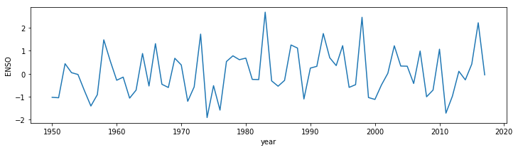
Exercise 1.2.9

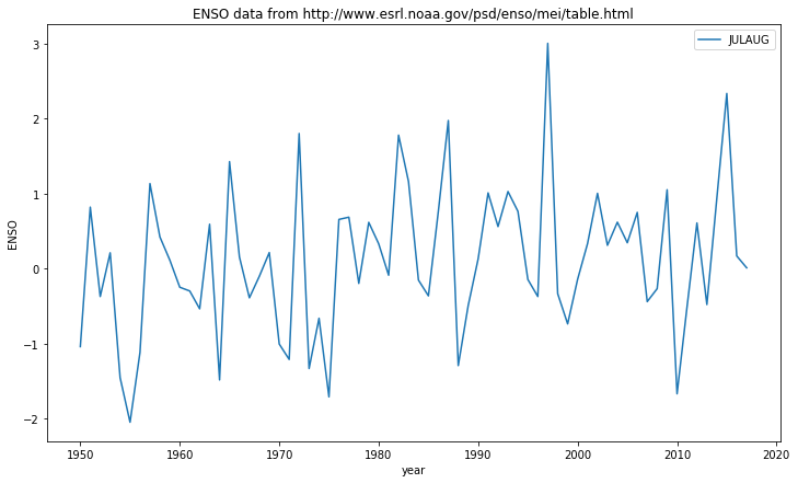
• use an implicit loop to create a list of ENSO values in a variable enso for the years 1950 up to last year for the period DECJAN.
• produce a plot of ENSO for DECJAN as a function of year (see below on how to do that).

Hint: check which column in the header is DECJAN. To start you off on this, we give you the implicit loop code for extracting the column containing the YEAR data (column 0). We also give you the code to achieve the plotting.

# do exercise here
# ANSWER

# generate a list called years of column 0 data
years = [all_float_data[row][0] for row in range(nrows)]

# very similar to aboive, but using column 1
enso = [all_float_data[row][1] for row in range(nrows)]

# for plotting
import pylab as plt
%matplotlib inline

#
plt.figure(0,figsize=(12,3))
plt.plot(years,enso)
plt.xlabel('year')
plt.ylabel('ENSO')

Text(0, 0.5, 'ENSO')

1.2.6 Summary

In section 1.2 you have been introduced to text representation in Python, as strings (type str), and shown that this sort of variable can be thought of an an ‘array’, and that it has a length attribute that can be accessed with len().

Other useful string manipulation methods you were introduced to are: replace(), find(), split() and splitlines(), though of course there are many more.

In an ‘array’, we can use an index to refer to a particular item (e.g. index 0 for the first item, 1 for the second, -1 for the last). We can use this idea to manipulate strings.

In a more general sense, we can take a ‘slice’ of an array, with the syntax [start:stop:skip] giving access to a regularly spaced part of an array. We can use this, for example, to print out every 10th value (skip=10).

You were also introduced to the idea of looping control structures, using a for ... in ...: statement, and the equivalent implicit form. This introduced the idea of indented code blocks and (related) nested structures (loops within loops).

In passing, you have also been shown how to pull html data from a URL (scraping) using the `requests <http://docs.python-requests.org/en/master/>`__ package, and also how to produce a simple data plot, using `pylab <https://matplotlib.org/index.html>`__.

1.3. Groups of things

Very often, we will want to group items together. There are several main mechanisms for doing this in Python, known as:

• string e.g. hello
• tuple, e.g. (1, 2, 3)
• list, e.g. [1, 2, 3]
• numpy array e.g. np.array([1, 2, 3])

A slightly different form of group is a dictionary:

• dict, e.g. {1:'one', 2:'two', 3:'three'}

You will notice that each of the grouping structures tuple, list and dict use a different form of bracket. The numpy array is fundamental to much work that we will do later.

We have dealt with the idea of a string as an ordered collection in the material above, so will deal with the others here.

We noted the concept of length (len()), that elements of the ordered collection could be accessed via an index, and came across the concept of a slice. All of these same ideas apply to the first set of groups (string, tuple, list, numpy array) as they are all ordered collections.

A dictionary is not (by default) ordered, however, so indices have no role. Instead, we use ‘keys’.

1.3.1 tuple

A tuple is a group of items separated by commas. In the case of a tuple, the brackets are optional. You can have a group of differnt types in a tuple (e.g. int, int, str, bool)

# load into the tuple
t = (1, 2, 'three', False)

# unload from the tuple
a,b,c,d = t

print(t)
print(a,b,c,d)

(1, 2, 'three', False)
1 2 three False

If there is only one element in a tuple, you must put a comma , at the end, otherwise it is not interpreted as a tuple:

t = (1)
print (t,type(t))
t = (1,)
print (t,type(t))

1 <class 'int'>
(1,) <class 'tuple'>

You can have an empty tuple though:

t = ()
print (t,type(t))

() <class 'tuple'>

E1.3.1 Exercise

• create a tuple called t that contains the integers 1 to 5 inclusive
• print out the value of t
• use the tuple to set variables a1,a2,a3,a4,a5

# do exercise here
# ANSWER

t = (1,2,3,4,5)
print(t)
a1,a2,a3,a4,a5 = t
print(a1,a2,a3,a4,a5)

(1, 2, 3, 4, 5)
1 2 3 4 5

1.3.2 list

A list is similar to a tuple. One main difference is that you can change individual elements in a list but not in a tuple. To convert between a list and tuple, use the ‘casting’ methods list() and tuple():

# a tuple
t0 = (1,2,3)

# cast to a list
l = list(t0)

# cast to a tuple
t = tuple(l)

print('type of {} is {}'.format(t,type(t)))
print('type of {} is {}'.format(l,type(l)))

type of (1, 2, 3) is <class 'tuple'>
type of [1, 2, 3] is <class 'list'>

You can concatenate (join) lists or tuples with the + operator:

l0 = [1,2,3]
l1 = [4,5,6]

l = l0 + l1
print ('joint list:',l)

joint list: [1, 2, 3, 4, 5, 6]

E1.3.2 Exercise * copy the code from the cell above, but instead of lists, use tuples * loop over each element in the tuple and print out the data type and value of the element

Hint: use a for ... in ... construct.

# do exercise here
# ANSWER

l0 = (1,2,3)
l1 = (4,5,6)

l = l0 + l1
print ('joint tuple:',l)

for t in l:
    print(type(t),t)

joint tuple: (1, 2, 3, 4, 5, 6)
<class 'int'> 1
<class 'int'> 2
<class 'int'> 3
<class 'int'> 4
<class 'int'> 5
<class 'int'> 6

A common method associated with lists or tuples is: * index()

Some useful methods that will operate on lists and tuples are: * len() * sort() * min(),max()

l0 = (2,8,4,32,16)

# print the index of the item integer 4
# in the tuple / list

item_number = 4

# Note the dot . here
# as index is a method of the class list
ind  = l0.index(item_number)

# notice that this is different
# as len() is not a list method, but
# does operatate on lists/tuples
# Note: do not use len as a variable name!
llen = len(l0)

# note the use of integers in the braces e.g. {0}
# rather than empty braces as before. This allows us to
# refer to particular items in the format argument list
print('the index of {0} in {1} is {2}'.format(item_number,l0,ind))
print('the length of the {0} {1} is {2}'.format(type(l0),l0,llen))

the index of 4 in (2, 8, 4, 32, 16) is 2
the length of the <class 'tuple'> (2, 8, 4, 32, 16) is 5

E1.3.3 Exercise

• copy the code to the block below, and test that this works with lists, as well as tuples
• find the index of the integer 16 in the tuple/list
• what is the index of the first item?
• what is the length of the tuple/list?
• what is the index of the last item?

# do exercise here
# ANSWER

# change this to a list
l0 = [2,8,4,32,16]

# print the index of the item integer 4
# in the tuple / list

item_number = 4

# Note the dot . here
# as index is a method of the class list
ind  = l0.index(item_number)

# notice that this is different
# as len() is not a list method, but
# does operatate on lists/tuples
# Note: do not use len as a variable name!
llen = len(l0)

# note the use of integers in the braces e.g. {0}
# rather than empty braces as before. This allows us to
# refer to particular items in the format argument list
print('the index of {0} in {1} is {2}'.format(item_number,l0,ind))
print('the length of the {0} {1} is {2}'.format(type(l0),l0,llen))

'''
find the index of the integer 16 in the tuple/list
what is the index of the first item?
what is the length of the tuple/list?
what is the index of the last item?
'''

print('16 is item number',l0.index(16))
print('the first item has index 0:',l0.index(2))
print('list length',len(l0))
print('the last item has index 4 (len - 1):',l0.index(16))

the index of 4 in [2, 8, 4, 32, 16] is 2
the length of the <class 'list'> [2, 8, 4, 32, 16] is 5
16 is item number 4
the first item has index 0: 0
list length 5
the last item has index 4 (len - 1): 4

A list has a much richer set of methods than a tuple. This is because we can add or remove list items (but not tuple).

• insert(i,j) : insert j beore item i in the list
• append(j) : append j to the end of the list
• sort() : sort the list

This shows that tuples and lists are ‘ordered’ (i.e. they maintain the order they are loaded in) so that indiviual elements may be accessed through an ‘index’. The index values start at 0 as we saw above. The index of the last element in a list/tuple is the length of the group, minus 1. This can also be referred to an index -1.

l0 = [2,8,4,32,16]

# insert 64 at the begining (before item 0)
# Note that this inserts 'in place'
# i.e. the list is changed by calling this
l0.insert(0,64)


# insert 128 *before* the last item (item -1)
l0.insert(-1,128)

# append 256 on the end
l0.append(256)

# copy the list
# and sort the copy
# Note the use of the copy() method here
# to create a copy
l1 = l0.copy()

# Note that this sorts 'in place'
# i.e. the list is changed by calling this
l1.sort()

print('the list {0} once sorted is {1}'.format(l0,l1))

the list [64, 2, 8, 4, 32, 128, 16, 256] once sorted is [2, 4, 8, 16, 32, 64, 128, 256]

E1.3.4 Exercise

• copy the above code and try out some different locations for inserting values (e.g. what does index -2 mean?)
• what happens if you take off the .copy() statement in the line l1 = l0.copy(), i.e. just use l1 = l0? Why is this?

# do exercise here
# ANSWER

l0 = [2,8,4,32,16]

# insert 64 at index -2 (2 from end)
# Note that this inserts 'in place'
# i.e. the list is changed by calling this
l0.insert(-2,64)
print(l0)

# copy the list
# and sort the copy
# Note the use of the copy() method here
# to create a copy
l1 = l0.copy()

# Note that this sorts 'in place'
# i.e. the list is changed by calling this
l1.sort()

print('the list {0} once sorted is {1}'.format(l0,l1))

[2, 8, 4, 64, 32, 16]
the list [2, 8, 4, 64, 32, 16] once sorted is [2, 4, 8, 16, 32, 64]

# do exercise here
# ANSWER

l0 = [2,8,4,32,16]

# insert 64 at index -2 (2 from end)
# Note that this inserts 'in place'
# i.e. the list is changed by calling this
l0.insert(-2,64)
print(l0)

# copy the list
# and sort the copy
# Note the use of the copy() method here
# to create a copy
l1 = l0

# Note that this sorts 'in place'
# i.e. the list is changed by calling this
l1.sort()

'''
Note that without the copy, we have altered l0
even though we did l1.sort()
'''

print('the list {0} once sorted is {1}'.format(l0,l1))

'''
For not in place sort, use sorted()
'''

l0 = [2,8,4,32,16]
print('the list {0} once sorted is {1}'.format(l0,sorted(l0)))

[2, 8, 4, 64, 32, 16]
the list [2, 4, 8, 16, 32, 64] once sorted is [2, 4, 8, 16, 32, 64]
the list [2, 8, 4, 32, 16] once sorted is [2, 4, 8, 16, 32]

1.3.3 np.array

An array is a group of objects of the same type. Because they are of the same type, they can be stored efficiently in compter memory, and also accessed efficiently.

Whilst there are different ways of forming arrays, the most common is to use numpy arrays, using the package numpy. To use this, we must first import the package into the current workspace. We do this with the import method. Using the optional as statement allows us to use a shorter (or more suitable) name for the package. We will generally call numpy np, so we use:

import numpy as np

to import (‘load’) the numpy package.

Often, we will read data from a file/URL as we did above for the ENSO dataset. In that case, we had to step through each item to convert from string form to floating point number.

This sort of thing is much more simply done using methods associated with numpy arrays.

A particularly useful numpy method is np.loadtxt(file) that loads an ASCII table of data straight into a numpy array.

Whilst this is designed to load data from a file, we can use io.StringIO() from the io package to make data that we already have as a string seem to np.loadtxt as if it were a file. This is a useful ‘trick’ for using methods that expect data in a file. The unpack=True option makes sure the data array is compoised the way we would expect it. The usecols option lets us select only those data columns we wish to read (0 and 1 here).

An alternative to np.loadtxt() is np.genfromtxt(). This has some additional features, such the invalid_raise flag. If this is set False, the loading is made somewhat tolerant to data errors (e.g. inconsistent number of columns). Further, we can explicitly set what will indicate missing_values in the input and what we would like to replace them with (filling_values) which can be useful for tidying up datasets.

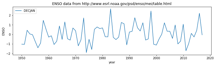
import requests
import numpy as np
import io

# access dataset as above
url = "http://www.esrl.noaa.gov/psd/enso/mei/table.html"
txt = requests.get(url).text

# copy the useful data
start_head = txt.find('YEAR')
start_data = txt.find('1950\t')
stop_data  = txt.find('2018\t')

# select a data column
data_column = 1

header = txt[start_head:start_data].split()
data = np.loadtxt(io.StringIO(txt[start_data:stop_data]),unpack=True,usecols=[0,data_column])

# so data[0] is the year data
#    data[1] is the enso data for column data_column
# print some attributes of the data array

print('array type',type(data))
print('data type',data.dtype)
print('number of dimensions',data.ndim)
print('data shape',data.shape)
print('data size',data.size)

# for plotting
import pylab as plt
%matplotlib inline

#
plt.figure(0,figsize=(12,3))
plt.plot(data[0],data[1],label=header[data_column])
plt.xlabel('year')
plt.ylabel('ENSO')
plt.title('ENSO data from {0}'.format(url))
plt.legend(loc='best')

array type <class 'numpy.ndarray'>
data type float64
number of dimensions 2
data shape (2, 68)
data size 136

<matplotlib.legend.Legend at 0x11b8b2668>

We saw in the example above that a numpy array (<class 'numpy.ndarray'>) has a set of attributes that include shape, ndim, dtype and size that we can use to query information about the array. We will learn morre about processing data with numpy arrays later in the course, but you should already see that they are a useful construct for manipulating multi-dimensional datasets.

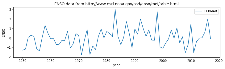
Exercise 1.3.4

• copy the code from the block above and modify it to plot the ENSO data for the period FEBMAR. Check this by looking at the data in the original table.
• modify the code to produce a plot of all periods (so the graph should have 12 lines, correctly labelled)

Hint: You will need to consider what, if anything to set of usecols (what happends if you don’t set usecols?) and provide a looping structure for the plotting.

# do exercise here
#ANSWER

import requests
import numpy as np
import io

# access dataset as above
url = "http://www.esrl.noaa.gov/psd/enso/mei/table.html"
txt = requests.get(url).text

# copy the useful data
start_head = txt.find('YEAR')
start_data = txt.find('1950\t')
stop_data  = txt.find('2018\t')

# select a data column
'''
Use column 3 for FEBMAR

The code is written so that we only need
change this one variable
'''
data_column = 3

header = txt[start_head:start_data].split()
data = np.loadtxt(io.StringIO(txt[start_data:stop_data]),unpack=True,usecols=[0,data_column])

# so data[0] is the year data
#    data[1] is the enso data for column data_column
# print some attributes of the data array

print('array type',type(data))
print('data type',data.dtype)
print('number of dimensions',data.ndim)
print('data shape',data.shape)
print('data size',data.size)

# for plotting
import pylab as plt
%matplotlib inline

#
plt.figure(0,figsize=(12,3))

plt.plot(data[0],data[1],label=header[data_column])
plt.xlabel('year')
plt.ylabel('ENSO')
plt.title('ENSO data from {0}'.format(url))
plt.legend(loc='best')

array type <class 'numpy.ndarray'>
data type float64
number of dimensions 2
data shape (2, 68)
data size 136

<matplotlib.legend.Legend at 0x11bcb0a20>

1.3.4 dict

The collections we have used so far have all been ordered. This means that we can refer to a particular element in the group by an index, e.g. array[10].

A dictionary is not (by default) ordered. Instead of indices, we use ‘keys’ to refer to elements: each element has a key associated with it. It can be very useful for data organisation (e.g. databases) to have a key to refer to, rather than e.g. some arbitrary column number in a gridded dataset.

A dictionary is defined as a group in braces (curley brackets). For each elerment, we specify the key and then the value, separated by :.

a = {'one': 1, 'two': 2, 'three': 3}

# we then refer to the keys and values in the dict as:

print ('a:\n\t',a)
print ('a.keys():\n\t',a.keys())     # the keys
print ('a.values():\n\t',a.values()) # returns the values
print ('a.items():\n\t',a.items())   # returns a list of tuples

a:
     {'one': 1, 'two': 2, 'three': 3}
a.keys():
     dict_keys(['one', 'two', 'three'])
a.values():
     dict_values([1, 2, 3])
a.items():
     dict_items([('one', 1), ('two', 2), ('three', 3)])

Because dictionaries are not ordered, we cannot guarantee the order they will come out in a for loop, but we will often use such a loop to iterate over the items in a dictionary.

for key,value in a.items():
    print(key,value)

one 1
two 2
three 3

We refer to specific items using the key e.g.:

print(a['one'])

1

You can add to a dictionary:

a.update({'four':4,'five':5})
print(a)

# or for a single value
a['six'] = 6
print(a)

{'one': 1, 'two': 2, 'three': 3, 'four': 4, 'five': 5}
{'one': 1, 'two': 2, 'three': 3, 'four': 4, 'five': 5, 'six': 6}

Quite often, you find that you have the keys you want to use in a dictionary as a list or array, and the values in another list.

In such a case, we can use the method zip(keys,values) to load into the dictionary. For example:

values = [1,2,3,4]
keys = ['one','two','three','four']

a = dict(zip(keys,values))

print(a)

{'one': 1, 'two': 2, 'three': 3, 'four': 4}

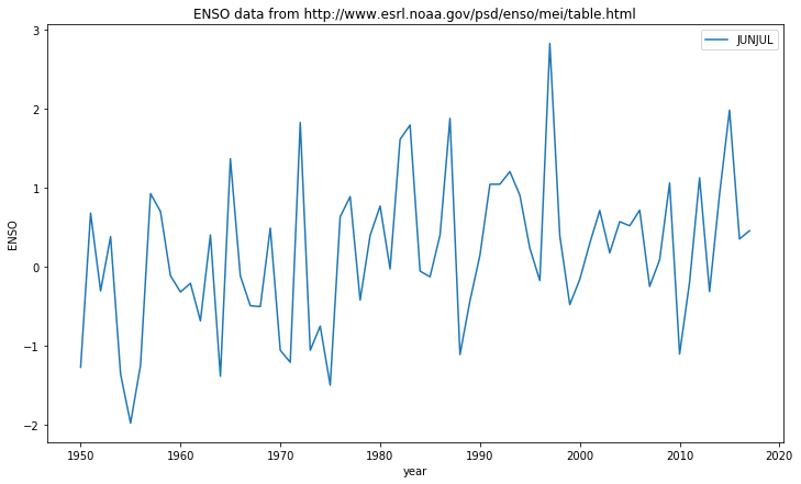
We will use this idea to make a dictionary of our ENSO dataset, using the items in the header for the keys. In this way, we obtain a more elegant representation of the dataset, and can refer to items by names (keys) instead of column numbers.

import requests
import numpy as np
import io

# access dataset as above
url = "http://www.esrl.noaa.gov/psd/enso/mei/table.html"
txt = requests.get(url).text

# copy the useful data
start_head = txt.find('YEAR')
start_data = txt.find('1950\t')
stop_data  = txt.find('2018\t')

header = txt[start_head:start_data].split()
data = np.loadtxt(io.StringIO(txt[start_data:stop_data]),unpack=True)

# use zip to load into a dictionary
data_dict = dict(zip(header, data))

key = 'MAYJUN'
# plot data
plt.figure(0,figsize=(12,7))
plt.title('ENSO data from {0}'.format(url))
plt.plot(data_dict['YEAR'],data_dict[key],label=key)
plt.xlabel('year')
plt.ylabel('ENSO')
plt.legend(loc='best')

<matplotlib.legend.Legend at 0x11bdc31d0>

Exercise 1.3.5

• copy the code above, and modify so that datasets for months ['MAYJUN','JUNJUL','JULAUG'] are plotted on the graph

Hint: use a for loop

# do exercise here
# ANSWER

import requests
import numpy as np
import io

# access dataset as above
url = "http://www.esrl.noaa.gov/psd/enso/mei/table.html"
txt = requests.get(url).text

# copy the useful data
start_head = txt.find('YEAR')
start_data = txt.find('1950\t')
stop_data  = txt.find('2018\t')

header = txt[start_head:start_data].split()
data = np.loadtxt(io.StringIO(txt[start_data:stop_data]),unpack=True)

# use zip to load into a dictionary
data_dict = dict(zip(header, data))


'''
Do the loop here
'''
for i,key in enumerate(['MAYJUN','JUNJUL','JULAUG']):
    # plot data
    '''
    Use enumeration i as figure number
    '''
    plt.figure(i,figsize=(12,7))
    plt.title('ENSO data from {0}'.format(url))
    plt.plot(data_dict['YEAR'],data_dict[key],label=key)
    plt.xlabel('year')
    plt.ylabel('ENSO')
    plt.legend(loc='best')

We can also usefully use a dictionary with a printing format statement. In that case, we refer directly to the key in ther format string. This can make printing statements much easier to read. We don;’t directly pass the dictionary to the fortmat staterment, but rather **dict, where **dict means “treat the key-value pairs in the dictionary as additional named arguments to this function call”.

So, in the example:

import requests
import numpy as np
import io

# access dataset as above
url = "http://www.esrl.noaa.gov/psd/enso/mei/table.html"
txt = requests.get(url).text

# copy the useful data
start_head = txt.find('YEAR')
start_data = txt.find('1950\t')
stop_data  = txt.find('2018\t')

header = txt[start_head:start_data].split()
data = np.loadtxt(io.StringIO(txt[start_data:stop_data]),unpack=True)

# use zip to load into a dictionary
data_dict = dict(zip(header, data))
print(data_dict.keys())

# print the data for MAYJUN
print('data for MAYJUN: {MAYJUN}'.format(**data_dict))

dict_keys(['YEAR', 'DECJAN', 'JANFEB', 'FEBMAR', 'MARAPR', 'APRMAY', 'MAYJUN', 'JUNJUL', 'JULAUG', 'AUGSEP', 'SEPOCT', 'OCTNOV', 'NOVDEC'])
data for MAYJUN: [-1.412e+00  2.880e-01 -7.560e-01  1.910e-01 -1.558e+00 -2.247e+00
 -1.523e+00  7.300e-01  8.120e-01 -6.200e-02 -2.870e-01 -1.850e-01
 -8.700e-01 -1.440e-01 -1.150e+00  8.670e-01 -1.930e-01 -2.360e-01
 -8.120e-01  8.010e-01 -6.360e-01 -1.420e+00  9.660e-01 -7.580e-01
 -6.940e-01 -1.148e+00  2.760e-01  4.140e-01 -6.050e-01  4.290e-01
  9.110e-01 -2.400e-02  9.300e-01  2.235e+00 -4.900e-02 -1.660e-01
  2.790e-01  1.958e+00 -5.820e-01 -2.420e-01  5.110e-01  1.051e+00
  1.735e+00  1.616e+00  8.030e-01  5.070e-01  8.700e-02  2.275e+00
  1.336e+00 -3.390e-01  1.000e-03  5.200e-02  9.320e-01  1.070e-01
  3.150e-01  5.890e-01  5.260e-01 -1.550e-01  1.420e-01  7.510e-01
 -2.280e-01 -3.000e-03  8.420e-01 -9.400e-02  1.046e+00  2.097e+00
  1.053e+00  1.039e+00]

The line print('data for MAYJUN: {MAYJUN}'.format(**data_dict)) is equivalent to writing:

print('data for {MAYJUN}'.format(YEAR=data_dict[YEAR],DECJAN=data_dict[DECJAN], ...))

In this way, we use the keys in the dictionary as keywords to pass to a method.

Another useful example of such a use of a dictionary is in saving a numpy dataset to file.

If the data are numpy arrays in a dictionary as above, we can store the dataset using:

import requests
import numpy as np
import io

# access dataset as above
url = "http://www.esrl.noaa.gov/psd/enso/mei/table.html"
txt = requests.get(url).text

# copy the useful data
start_head = txt.find('YEAR')
start_data = txt.find('1950\t')
stop_data  = txt.find('2018\t')

header = txt[start_head:start_data].split()
data = np.loadtxt(io.StringIO(txt[start_data:stop_data]),unpack=True)

# use zip to load into a dictionary
data_dict = dict(zip(header, data))

filename = 'enso_mei.npz'

# save the dataset
np.savez_compressed(filename,**data_dict)

What we load from the file is a dictionary-like object <class 'numpy.lib.npyio.NpzFile'>.

If needed, we can cast this to a dictionary with dict(), but it is generally more efficient to keep the original type.

# load the dataset

filename = 'enso_mei.npz'

loaded_data = np.load(filename)

print(type(loaded_data))

# test they are the same using np.array_equal
for k in loaded_data.keys():
    print('\t',k,np.array_equal(data_dict[k], loaded_data[k]))

<class 'numpy.lib.npyio.NpzFile'>
     YEAR True
     DECJAN True
     JANFEB True
     FEBMAR True
     MARAPR True
     APRMAY True
     MAYJUN True
     JUNJUL True
     JULAUG True
     AUGSEP True
     SEPOCT True
     OCTNOV True
     NOVDEC True

Exercise 1.3.6

• Using what you have learned above, access the Met Office data file `https://www.metoffice.gov.uk/hadobs/hadukp/data/monthly/HadSEEP_monthly_qc.txt <https://www.metoffice.gov.uk/hadobs/hadukp/data/monthly/HadSEEP_monthly_qc.txt>`__ and create a ‘data package’ in a numpy.npz file that has keys of YEAR and each month in the year, with associated datasets of Monthly Southeast England precipitation (mm).
• confirm that tha data in your npz file is the same as in your original dictionary
• produce a plot of October rainfall using these data for the years 1900 onwards

# do exercise here
# ANSWER

'''
Exploration of dataset shows:


Monthly Southeast England precipitation (mm). Daily automated values used after 1996.
Wigley & Jones (J.Climatol.,1987), Gregory et al. (Int.J.Clim.,1991)
Jones & Conway (Int.J.Climatol.,1997), Alexander & Jones (ASL,2001). Values may change after QC.
YEAR   JAN   FEB   MAR   APR   MAY   JUN   JUL   AUG   SEP   OCT   NOV   DEC   ANN
 1873  87.1  50.4  52.9  19.9  41.1  63.6  53.2  56.4  62.0  86.0  59.4  15.7  647.7
 1874  46.8  44.9  15.8  48.4  24.1  49.9  28.3  43.6  79.4  96.1  63.9  52.3  593.5

so we have 3 lines of header
then the column titles
then the data

we can define these as before using

txt.find('YEAR')
start_data = txt.find('1873')
stop_data = None


Other than the filenames then, the code
is identical
'''

import requests
import numpy as np
import io

# access dataset as above
url = "https://www.metoffice.gov.uk/hadobs/hadukp/data/monthly/HadSEEP_monthly_qc.txt"
txt = requests.get(url).text

# copy the useful data
start_head = txt.find('YEAR')
start_data = txt.find('1873')
stop_data  = None

header = txt[start_head:start_data].split()
data = np.loadtxt(io.StringIO(txt[start_data:stop_data]),unpack=True)

# use zip to load into a dictionary
data_dict = dict(zip(header, data))

filename = 'HadSEEP_monthly_qc.npz'

# save the dataset
np.savez_compressed(filename,**data_dict)

# ANSWER

loaded_data = np.load(filename)

print(type(loaded_data))

# test they are the same using np.array_equal
for k in loaded_data.keys():
    print('\t',k,np.array_equal(data_dict[k], loaded_data[k]))

<class 'numpy.lib.npyio.NpzFile'>
     YEAR True
     JAN True
     FEB True
     MAR True
     APR True
     MAY True
     JUN True
     JUL True
     AUG True
     SEP True
     OCT True
     NOV True
     DEC True
     ANN True

# ANSWER

'''
October rainfall, 1900+
'''

year = loaded_data['YEAR']

# mask where years match
mask = year  >= 1900

oct = loaded_data['OCT']

# set invalid data points to nan
oct[oct<0] = np.nan

plt.plot(year[mask],oct[mask])

[<matplotlib.lines.Line2D at 0x11c76a9e8>]

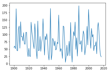
1.3.5 Summary

In this section, we have extended the types of data we might come across to include groups . We dealt with ordered groups of various types (tuple, list), and introduced the numpy package for numpy arrays (np.array). We saw dictionaries as collections with which we refer to individual items with a key.

We learned in the previous section how to pull apart a dataset presented as a string using loops and various using methods and to construct a useful dataset ‘by hand’ in a list or similar structure. It is useful, when learning to program, to know how to do this.

Here, we saw that packages such as numpy provide higher level routines that make reading data easier, and we would generally use these in practice. We saw how we can use zip() to help load a dataset from arrays into a dictionary, and also the value of using a dictionary representation when saving numpy files.