# All imports go here. Run me first!
import datetime
from pathlib import Path  # Checks for files and so on
import numpy as np  # Numpy for arrays and so on
import pandas as pd
import sys
import matplotlib.pyplot as plt  # Matplotlib for plotting
# Ensure the plots are shown in the notebook
%matplotlib inline

import gdal
import osr
import numpy as np

from geog0111.geog_data import procure_dataset

if not Path("data/mod14_data").exists():
    _ = procure_dataset("mod14_data", destination_folder="data/mod14_data")
else:
    print("Data already available")

Data already available

Group project: Fire and teleconnections¶

There is much public and scientific interest in monitoring and predicting the activity of wildfires and such topics are often in the media, or here for a more recent event.

Part of this interest stems from the role fire plays in issues such as land cover change, deforestation and forest degradation and Carbon emissions from the land surface to the atmosphere, but also of concern are human health impacts, effects on soil, erosion, etc. The impacts of fire should not however be considered as wholy negative, as it plays a significant role in natural ecosystem processes.

For many regions of the Earth, there are large inter-annual variations in the timing, frequency and severity of wildfires. Whilst anthropogenic activity accounts for a large proportion of fires started, this is not in itself a new phenomenon, and fire has been and is used by humans to manage their environment.

Fires spread where: (i) there is an ignition source (lightning or man, mostly); (ii) sufficient combustible fuel to maintain the fire. The latter is strongly dependent on fuel loads and moisture content, as well as meteorological conditions. Generally then, when conditions are drier (and there is sufficient fuel and appropriate weather conditions), we would expect fire spread to increase. If the number of ignitions remained approximately constant, this would mean more fires. Many models of fire activity predict increases in fire frequency in the coming decades, although there may well be different behaviours in different parts of the world.

Here’s Richard Feynman talking about fire and the carbon cycle.

from IPython.display import YouTubeVideo
YouTubeVideo('ITpDrdtGAmo')

Satellite data has been able to provide us with increasingly useful tools for monitoring wildfire activity, particularly since 2000 with the MODIS instruments on the NASA Terra and Aqua (2002) satellites. A suite of ‘fire’ products have been generated from these data that have been used in a large number of publications and practical/management projects.

There is growing evidence of ‘teleconnection’ links between fire occurence and large scale climate patterns, such as ENSO.

The proposed mechanisms are essentially that such climatic patterns are linked to local water status and temperature and thus affect the ability of fires to spread. For some regions of the Earth, empirical models built from such considerations have quite reasonable predictive skill, meaning that fire season severity might be predicted some months ahead of time.

In this Session..¶

In this session, you will be working in groups (of 3 or 4) to build a computer code in Python to explore links between fire activity and Sea Surface Temperature anomalies.

This is a team exercise, but does not form part of your formal assessment for this course. You should be able to complete the exercise in a 3-4 hour session, if you work effectively as a team. Staff will be on hand to provide pointers.

You should be able to complete the exercise using coding skills and python modules that you have previously experience of, though we will also provide some pointers to get you started.

In a nutshell, the goal of this exercise is

Using monthly fire count data from MODIS Terra, develop and test a predictive model for the number of fires per unit area per year driven by Sea Surface Temperature anomaly data.

The datasets should be created at 5 degree resolution on a latitude/longitude grid, as climate patterns will probably show some sort of response at broader spatial scales.

You should concentrate on building the model that predicts peak fire count in a particular year at a particular location, i.e. derive your model for annual peak fire count.

Datasets¶

We suggest that the datasets you use of this analysis, following Chen at al. (2011), are:

MODIS Terra fire counts (2001-2011) (MOD14CMH). The particular dataset you will want from the file is ‘SUBDATASET_2 [360x720] CloudCorrFirePix (16-bit integer)’.
Climate index data from NOAA (e.g. see this list)

If you ever wish to take this study further, you can find various other useful datasets such as these.

Fire Data¶

The MOD14CMH CMG data are available from the UMD ftp server but have also been packaged for you and can be imported using the following code (this has already been done in the first imports cell above):

from geog0111.geog_data import procure_dataset

_ = procure_dataset("mod14_data",
                destination_folder="data/mod14_data")

The data are in HDF format, and you ought to be able to read them nto numpy arrays an operate with them. Note that there is data for MODIS TERRA and AQUA sensors, and if you want to use them together, you need to figure out the overlap period (AQUA only started providing data halfway through 2002).

The teleconnections data¶

Teleconnections data are available from a large number of places on the internet. You can find some sources of inspiration here. The data can be processed in two different ways: either as it is, or as anomalies (where you define a baseline temporal period, calculate some average value, and look at the residual between the actual index and the historical average). It’s up to you what index you may want to use, and whether you want to use anomalies or directly the index value.

The predictive model¶

The model is very simple: we assume that the there is a linear relationship between the teleconnection at some given lag, and the recorded number of thermal anomalies. Bear in mind that the aim is to predict fire counts some months in advance using a teleconnection. As pseudo-code, for a pixel location i,j, you’d have something like this:

i, j # this is the pixel value
# Read in the peak fire month
peak_fire_month = get_peak_fire_month(i, j)
# Read in peak fire counts for all years for the pixel of interest
y = get_all_fire_counts_for_all_years(i, j)
# Loop over some lags
for lag in 0, ..., 12
do
    # Get the lagged teleconnection
    x = get_teleconnection_for_all_years(peak_fire_month - lag)
    # Perform linear regression and store the results
    m[lag], c[lag], r2[lag] = linear_regression(x, y)
done
best_lag = argmax(r2) # Select best lag
store_model(i, j, best_lag, m[best_lag], c[best_lag], r2[best_lag])

Splitting the tasks¶

You may want to assign tasks to individual members of the group. A reasonable split might be

One person is responsible for the satellite data. This includes creating a 5 degree global resolution monthly dataset, and from it, derive for each grid cell, a peak fire month dataset, as well as a dataset with the fire counts at each peak fire month for all available years (more hints below)
Another person might be in charge for getting hold of the teleconnections dataset, and process it into a suitable array
Finally, some other person could be in charge of combining both fire counts and teleconnections datasets together and developing and testing a linear model to predict fire counts.

The satellite fire counts data¶

You should probably start using the TERRA data. Files are named MOD14CMH.YYYYMM.005.01.hdf. By now, you should be familiar with the naming convention, and figure out that YYYYMM is the year and month the dataset refers to.
Remember that this is a dataset of fire counts. You may want to check for weird data (e.g. can fire counts be less than zero?)

The satellite data need to be aggregated to a coarser resolution of 5 degrees. This means that you have to sum the fire counts for every 10x10 original pixels, discarding missing values and so on. There’s two ways of doing this: a loop and an array-based one.

Loop based aggregation

for i in range(int(nx/size)):
   for j in range(int(ny/size)):
       aggregated[i,j] = aggregate_function(original_data[i*size:((i+1)*size),
                                                          j*size:((j+1)*size)])

Array based aggregation: If the window size fits neatly in the data, you can just reshape the array and aggregate over as

aggregated = aggregate_function(original_data.reshape(
                                (nx/nsize, nsize, ny/nsize, nsize)),
                                axis=(1,3))

You ought to discard 2000 as there are only two months of data available for that year.
A reasonable data model for this is a numpy array of size n_months*n_years, nn, mm. You may also want to store the months and years as a 2D array (e.g. n_months*n_years,2)
Once you have this, you can loop over your fire array, selecting all the fire counts for each year (e.g. 12 numbers) for each pixel, and finding the location of the maximum (using e.g. np.argmax). You’ll end up with an array of size n_years, nn, mm.
So now you need to decide which month is, on average, the peak fire month. How could you do this? The mean is problematic, as you may end up with something like e.g. 6.5. Are there other statistical metrics that might results useful (e.g. see this)?

At this point, you should end up with one main array of size nn, mm (e.g. 36, 72), where every grid cell is populated by the peak fire number defined from the data, as well as the n_years,nn,nn array with the fire counts at peak fire month. Make sure it is clear what you mean by month number!!! Note that we also have data available for the AQUA platform, and you may want to use it too.

If you plot them, they should look like this:

The teleconnections¶

You can start with one teleconnection, but you may want to explore others.
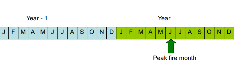
A data structure for the telecon data that might be useful and convenient is to stack two consecutive years together. It then makes it easy to loop over different lags (e.g. if your peak fire month for a pixel is February, then examining the 12 previous months can be done by looking at positions 13 (Feb), 12 (Jan), 11 (Dec previous year) and so on. Here’s how it looks like graphically

With this in mind, you should aim to have an array with your teleconnection (or a dictionary of teleconnections!) with size n_years*24.

You can use the ESRL NOAA webpage to plot time series of your index (… indices) of choice, and make sure you have processed the data correctly.

Developing the model¶

The model is a simple linear model that relates the teleconnection value at some lag \(l\) with respect to the peak fire month (\(tc_{l}\)) with the number of fire counts for a given cell, \(N_{counts,\,i,j}\)

\[m\cdot tc_{l} + c = N_{counts,\,i,j}\]

You have to split the data into a testing and training set: select a number of years to fit the model, and another one to test the model.
The training will produce estimates of the slope \(m\) and intercept \(c\) for every pixel and time lag \(l\).
There are different ways to select the best lag, but the simplest one could be in terms of the coefficient of determination \(r^2\): just choose the highest!
You should store the per grid cell model parameters, as well as probably the \(r^2\) (why?), and the optimal lag.

You can see an example of how this works on a particular grid cell in the following plot

Model testing¶

The previous plot shows that for a particular grid cell, the model is very succesful in the training phase (open orange circles), but the predictive phase is a bit of a mixed bag, with half the predictions being an important underestimate. However, this is a single cell validation. You ought to think of how to best validate the model. Scatter plots similar to the one above are useful, but maybe you have other ideas.

A useful test of the robustness of the model in the light of limited data is to use bootstrapping: a fraction of the dataset (e.g. a few years) are left out for testing as you’ve done above, but the procedure is repeated by replacing the training and testing datasets, to give you a distribution of the predictive performance of the model. There is a practical and very readable introduction to bootstrapping here

You may want to pack all the model development, teleconnection gathering and analysis in one top-level function that allows you to quickly repeat the fitting and testing procedure using different sets of years.