# All imports go here. Run me first!
import datetime
from pathlib import Path  # Checks for files and so on
import numpy as np  # Numpy for arrays and so on
import pandas as pd
import sys
import matplotlib.pyplot as plt  # Matplotlib for plotting
# Ensure the plots are shown in the notebook
%matplotlib inline

import gdal
import osr
import numpy as np

from geog0111.geog_data import procure_dataset
%matplotlib inline

Fitting models of phenology to MODIS LAI data

In the previous Section, we have looked at a very simple model of phenology, probably applicable to a lot of deciduous vegetation. We have created some synthetic data, and we have tried to fit the model to these “pseudo observations”. It is now the time to extract time series of MODIS data, and try to fit the model to them.

In this Section, we’ll use some of the work we used before. In particular, we’ll use a mosaic of LAI over Western Europe derived from the MODIS MCD15 product. The product has already been packed in an easy to use GeoTIFF file, together with the corresponding QA dataset. We’ll define some functions here again (they are from other sections, but added here for simplicity):

The phenology model

The phenology model is the double logistic/sigmoid curve, given by

\[y = p_0 - p_1\cdot\left[\frac{1}{1+\exp\left(p_2\cdot(t-p_3)\right)} + \frac{1}{1+\exp\left(-p_4\cdot(t-p_5)\right)} - 1\right].\]

We also define a cost function for it based on observations of LAI, uncertainty and a mask to indicate missing observations.

def dbl_sigmoid_function(p, t):
    """The double sigmoid function defined over t (where t is an array).
    Takes a vector of 6 parameters"""

    sigma1 = 1./(1+np.exp(p[2]*(t-p[3])))
    sigma2 = 1./(1+np.exp(-p[4]*(t-p[5])))
    y = p[0] - p[1]*(sigma1 + sigma2 - 1)
    return y

def cost_function(p, t, y_obs, passer, sigma_obs, func=dbl_sigmoid_function):
    y_pred = func(p, t)
    cost = -0.5* (y_pred[passer]-y_obs)**2/sigma_obs**2
    return -cost.sum()

Interpreting the QA LAI data

From before, we interpret the QA layer in the MODIS product by looking at bits 5 to 7, and turning them into a weight given by \(\phi^{QA}\), where \(\phi\) is the golden ratio \((=0.618\dots)\), and \(QA\) can take values between 0 and 3, indicating a decreasing quality in the retrieval, and hence, a lower weight.

def get_sfc_qc(qa_data, mask57 = 0b11100000):
    sfc_qa = np.right_shift(np.bitwise_and(qa_data, mask57), 5)
    return sfc_qa

def get_scaling(sfc_qa, golden_ratio=0.61803398875):
    weight = np.zeros_like(sfc_qa, dtype=np.float)
    for qa_val in [0, 1, 2, 3]:
        weight[sfc_qa == qa_val] = np.power(golden_ratio, float(qa_val))
    return weight

Selecting data from a raster file

In this activity, we want to select a pixel in the map and read in the data for all time steps. This can be achieved by plotting the map with e.g. imshow, and judiciously selecting a row and a column. However, in many cases, we have locations of interest as a list of latitude and longitude pairs. These do not automatically map to rows and columns, because the the MODIS data are projected in a projection that is not latitude/longitude. So the process of going from latitude-longitude pair to row and column needs two steps: converting latitude-longitude coordinates into the coordinates of the raster of interest (in the case of MODIS, MODIS sinusoidal projection), and then converting the raster coordinates into pixel numbers.

Converting geographic projections

Converting from latitude-longitude pairs (or any other representation) into a different projection can be accomplished by GDAL (surprise!). We first need to find a way to defining the projection. There are several ways to do this:

• EPSG codes These are numerical codes that have been internationally agreed and fully define a projection
• Proj4 strings Proj4 is the library the manages coordinate conversions under the hood in GDAL. It has a method to define a projection as a text string.
• WKT (Well-known text) format This is a standard that defines the projection as a text block

Generally speaking, their simplicity of use recommends EPSG, a single number. In some cases, proj4 strings are best (e.g. for some product-specific projections), and WKT is generally used by other GIS software.

In any case, the spatialreference website provides a convenient “Rosetta stone” of projections in these different conventions.

Use spatialreference.org to find out what projection the EPSG code 4326 corresponds to

In Python, using the OSR part of the GDAL library, we define the source and destinations projections using SpatialReference objects, which are then populated with e.g. EPSG codes or proj4 strings:

import osr
# Define the Lat/Long object
wgs84 = osr.SpatialReference()
# In this case, we use EPSG code
wgs84.ImportFromEPSG(4326)
# Define the MODIS projection object
modis_sinu = osr.SpatialReference()
# In this case, we use the proj4 string
modis_sinu.ImportFromProj4("+proj=sinu +lon_0=0 +x_0=0 +y_0=0 " +
                       "+a=6371007.181 +b=6371007.181 +units=m +no_defs")

The previous code snippet defines two SpatialReference objects. These can be used to map from MODIS to/and from Latitude Longitude (or “WGS84”) coordinates by using the osr.CoordinateTransformation object:

transformation = osr.CoordinateTransformation(wgs84, modis_sinu)
modis_x, modis_y, modis_z = transformation.TransformPoint(longitude,
                                                          latitude)

Clearly, changing the order of the parameters in osr.CoordinateTransformation would reverse the transformation.

Write some python code to convert the location of the Pearson Building (latitude: 51.524750 decimal degrees, longitude=-0.134560 decimal degrees) between WGS84 and OSGB 1936/British National Grid and UTM zone 30N/WGS84. Use mygeodata.cloud to test that your results are sensible

import osr

lat, lon = 51.524750, -0.134560
wgs84 = osr.SpatialReference()
wgs84.ImportFromEPSG(4326)
osgb = osr.SpatialReference()
osgb.ImportFromEPSG(27700)
utm30n = osr.SpatialReference()
utm30n.ImportFromEPSG(32630)

transformation_osgb = osr.CoordinateTransformation(wgs84, osgb)
transformation_utm = osr.CoordinateTransformation(wgs84, utm30n)
print("GDAL OSGB: ", transformation_osgb.TransformPoint(lon, lat))
print("Expected OSGB: 529510.455794 182297.498731")
print("GDAL UTM30N/WGS84: ", transformation_utm.TransformPoint(lon, lat))
print("Expected UTM30N/WGS84: 698771.632126 5712074.37524")

GDAL OSGB:  (529510.4529047138, 182297.49865122623, -46.15269147325307)
Expected OSGB: 529510.455794 182297.498731
GDAL UTM30N/WGS84:  (698771.6321257285, 5712074.3752355995, 0.0)
Expected UTM30N/WGS84: 698771.632126 5712074.37524

Finding a pixel based on its coordinates

Geospatial data usually contain a definition of how to go from a coordinate to a pixel location. In GDAL, the generic way this is encoded is through the GeoTransform element, a six element vector that details the location of the Upper Left corner of the raster file (pixel position (0, 0)), the pixel spacing, as well as a possible angular shift. Here are the elements of the geotransform array:

1. The Upper Left easting coordinate (i.e., horizontal)
2. The E-W pixel spacing
3. The rotation (0 degrees if image is “North Up”)
4. The Upper left northing coordinate (i.e., vertical)
5. The rotation (0 degrees)
6. The N-S pixel spacing, negative as we will be counting from the UL corner

With this in mind, and remembering that in Python arrays start at 0, and ignoring the rotation contributions, the pixel numbers can be calculated as follows

 pixel_x = (x_location - geo_transform[0])/geo_transform[1] \
     # The difference in distance between the UL corner (geot[0] \
     #and point of interest. Scaled by geot[1] to get pixel number

pixel_y = (y_location - geo_transform[3])/(geo_transform[5]) # Like for pixel_x, \
     #but in vertical direction. Note the different elements of geot \
     #being used

Since it’s easy to get this wrong, GDAL provides a couple of methods to do this conversion directly:

inv_geoT = gdal.InvGeoTransform(geotransform)
r, c = (gdal.ApplyGeoTransform(inv_geoT, x_location, y_location))

Let’s see a whole example of this zooming in the fAPAR map from the MODIS MCD15 product near the fine city of A Coruña in Galicia, NW Spain (latitude: 43.3623, longitude: -8.4115):

%%html
<iframe src="https://www.google.com/maps/embed?pb=!1m14!1m12!1m3!1d238659.69294928786!2d-8.664931741126212!3d43.39317238062582!2m3!1f0!2f0!3f0!3m2!1i1024!2i768!4f13.1!5e1!3m2!1sen!2suk!4v1542817273641" width="600" height="450" frameborder="0" style="border:0" allowfullscreen></iframe>

##################################################################
# Define transformations and variables. This is like above!
##################################################################

y_location, x_location = 43.3623, -8.4115 # In degs
# Define the Lat/Long object
wgs84 = osr.SpatialReference()
# In this case, we use EPSG code
wgs84.ImportFromEPSG(4326)
# Define the MODIS projection object
modis_sinu = osr.SpatialReference()
# In this case, we use the proj4 string
modis_sinu.ImportFromProj4("+proj=sinu +lon_0=0 +x_0=0 +y_0=0 " +
                           "+a=6371007.181 +b=6371007.181 +units=m +no_defs")

transformation = osr.CoordinateTransformation(wgs84, modis_sinu)
modis_x, modis_y, modis_z = transformation.TransformPoint(x_location,
                                                         y_location)
print("MODIS coordinates: ", modis_x, modis_y)

##################################################################
# We use a random file in the UCL filesystem
##################################################################

fname = "/home/plewis/public_html/geog0111_data/lai_files/" + \
              "MCD15A3H.A2016273.h17v04.006.2016278070708.hdf"
g = gdal.Open('HDF4_EOS:EOS_GRID:"%s":MOD_Grid_MCD15A3H:Fpar_500m' % fname)


##################################################################
# This is where new stuff begins
# Find out the pixel location from the MODIS Easting & Northing
##################################################################

geoT = g.GetGeoTransform()
inv_geoT = gdal.InvGeoTransform(geoT)
r, c = (gdal.ApplyGeoTransform(inv_geoT, modis_x, modis_y))
r = int(r+0.5)
c = int(c+0.5)
print("Pixel location: ", r,c)

##################################################################
# Now, read in the data, and plot it
##################################################################

fapar = g.ReadAsArray()/100
fapar[fapar>1] = np.nan
cmap = plt.cm.inferno
cmap.set_bad("0.6")
plt.figure(figsize=(8, 8))
plt.imshow(fapar, interpolation="nearest", vmin=0, vmax=1, cmap=cmap)
plt.colorbar()

##################################################################
# Plot a zoomed-in version
##################################################################


plt.figure(figsize=(8, 8))
plt.imshow(fapar[(c-50):(c+50), (r-50):(r+50)], interpolation="nearest",
           vmin=0, vmax=1, cmap=cmap)
plt.colorbar()

MODIS coordinates:  -680000.4782137175 4821673.202327191
Pixel location:  932 1593

<matplotlib.colorbar.Colorbar at 0x7f8ffdcf6390>

/home/ucfajlg/miniconda3/envs/python3/lib/python3.6/site-packages/matplotlib/font_manager.py:1328: UserWarning: findfont: Font family ['sans-serif'] not found. Falling back to DejaVu Sans
  (prop.get_family(), self.defaultFamily[fontext]))

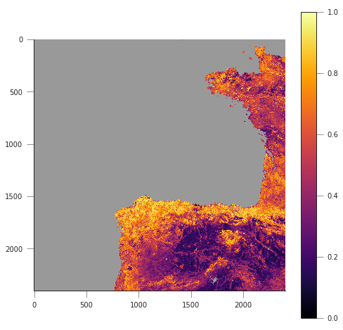
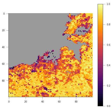
We can see that in the example above, we’re getting the right pixel number. Clearly, the code above is a bit of a mess, and needs to be cleaned up, split into functions and tested. This is an example, and you can take this as a reference of how to document functions etc.

def convert_coordinates(x_location, y_location,
                       src_transform={'EPSG':4326},
                       dst_transform={'Proj4':
                                           "+proj=sinu +lon_0=0 +x_0=0 " +
                                           "+y_0=0 +a=6371007.181 " +
                                           "+b=6371007.181 +units=m +no_defs"
                                          }):
    """A function to convert coordinates from one target coordinate
    representation to another. The input an output transformation can be given
    in either EPSG codes or Proj4 strings, by providing the function with a
    dictionary with the desired convention as a key, and with the relevant
    codes as its only element.

    Parameters
    ----------
    x_location: float
        The x location
    y_location: float
        The y location
    src_transform: dict
        A dictionary with keys either "EPSG" or "Proj4" (anything else throws
        an exception) with the description of the **input** projection
    dst_transform: dict
        A dictionary with keys either "EPSG" or "Proj4" (anything else throws
        an exception) with the description of the **output** projection
    Returns
    --------

    The transformed x and y coordinates"""
    input_coords = osr.SpatialReference()
    # In this case, we use EPSG code
    try:
        input_coords.ImportFromEPSG(src_transform["EPSG"])
    except KeyError:
        input_coords.ImportFromProj4(src_transform["Proj4"])
    except KeyError:
        raise ValueError("src_transform not dictionary with EPSG/Proj4 keys!")


    output_coords = osr.SpatialReference()
    try:
        output_coords.ImportFromEPSG(dst_transform["EPSG"])
    except KeyError:
        output_coords.ImportFromProj4(dst_transform["Proj4"])
    except KeyError:
        raise ValueError("src_transform not dictionary with EPSG/Proj4 keys!")


    transformation = osr.CoordinateTransformation(input_coords,
                                                 output_coords)
    output_x, output_y, output_z = transformation.TransformPoint(x_location,
                                                         y_location)
    return output_x, output_y


##################################################################
# Test function
##################################################################

y_location, x_location = 43.3623, -8.4115 # In WGS84
print (convert_coordinates(x_location, y_location))

(-680000.4782137175, 4821673.202327191)

def get_pixel(raster, point_x, point_y):
    """Get the pixel for given coordinates (in the raster's convention, not
    checked!) for a raster file.

    Parameters
    ----------
    raster: string
        A GDAL-friendly raster filename
    point_x: float
        The Easting in the same coordinates as the raster (not checked!)
    point_y: float
        The Northing in the same coordinates as the raster (not checked!)

    Returns
    -------
    The row/column (or column/row, depending on how you define it)
    """
    g = gdal.Open(raster)
    if g is None:
        raise ValueError(f"{raster:s} cannot be opened!")
    geoT = g.GetGeoTransform()
    inv_geoT = gdal.InvGeoTransform(geoT)
    r, c = (gdal.ApplyGeoTransform(inv_geoT, point_x, point_y))
    return int(r + 0.5), int(c + 0.5)

##################################################################
# Test function
##################################################################


fname = "/home/plewis/public_html/geog0111_data/lai_files/" + \
              "MCD15A3H.A2016273.h17v04.006.2016278070708.hdf"
gdal_fname = 'HDF4_EOS:EOS_GRID:"%s":MOD_Grid_MCD15A3H:Fpar_500m' % fname
print (get_pixel(gdal_fname, -680000.4782137175, 4821673.202327191))

(932, 1593)

Retrieving a time series from a multi-band raster

We have produced 4 rasters, with the LAI value for 2016 and 2017, as well as the correspodingn FparLai_QC layer. They’re avaialable in data/euro_lai. Let’s quickly have a look at the data:

success = procure_dataset("euro_lai", destination_folder="data/euro_lai/",
                         verbose=True)
if not success:
    print("Something happened copying files across to data/euro_lai")

print(gdal.Info("data/euro_lai/Europe_mosaic_Lai_500m_2017.tif").split("\n")[:10])

Running on UCL's Geography computers
trying /archive/rsu_raid_0/plewis/public_html/geog0111_data
trying /data/selene/ucfajlg/geog0111_data/lai_data/
trying /data/selene/ucfajlg/geog0111_data/
Linking /data/selene/ucfajlg/geog0111_data/euro_lai/Europe_mosaic_FparLai_QC_2016.tif to data/euro_lai/Europe_mosaic_FparLai_QC_2016.tif
Linking /data/selene/ucfajlg/geog0111_data/euro_lai/Europe_mosaic_FparLai_QC_2017.tif to data/euro_lai/Europe_mosaic_FparLai_QC_2017.tif
Linking /data/selene/ucfajlg/geog0111_data/euro_lai/Europe_mosaic_Lai_500m_2016.tif to data/euro_lai/Europe_mosaic_Lai_500m_2016.tif
Linking /data/selene/ucfajlg/geog0111_data/euro_lai/Europe_mosaic_Lai_500m_2017.tif to data/euro_lai/Europe_mosaic_Lai_500m_2017.tif
['Driver: GTiff/GeoTIFF', 'Files: data/euro_lai/Europe_mosaic_Lai_500m_2017.tif', 'Size is 4800, 4800', 'Coordinate System is:', 'PROJCS["unnamed",', '    GEOGCS["Unknown datum based upon the custom spheroid",', '        DATUM["Not_specified_based_on_custom_spheroid",', '            SPHEROID["Custom spheroid",6371007.181,0]],', '        PRIMEM["Greenwich",0],', '        UNIT["degree",0.0174532925199433]],']

We have 90 (or 91) layers, from day 1 to day 360/364 in the year. While we could read all the data in memory, it’s wasteful of resources, and we might as well try to read in all the bands for a given pixel.

We can do this with the read_tseries function below. Basically, we this function calls the previous pixel-location functions, and then reads the entire time series for a pixel in one go. The function is defined below:

#def get_pixel(raster, point_x, point_y):
#def convert_coordinates(x_location, y_location,


def read_tseries(raster, lat, long):
    """Read a time series (or all bands) for a raster file given latitude and
    longitude coordinates.
    **NOTE** Only works with Byte/UInt8 data types!
    """
    g = gdal.Open(raster)
#   px, py = get_pixel(raster, *convert_coordinates(x_location,
#                                                   y_location))
#    tmpx, tmpy =convert_coordinates(long, lat)
#    px, py = get_pixel(raster, tmpx, tmpy)

    px, py = get_pixel(raster, *convert_coordinates(long, lat))
    print(px, py)
    if 0 <= px >= g.RasterXSize:
        raise ValueError(f"Point outside of raster ({px:d}/{g.RasterXSize:d})")
    if 0 <= py >= g.RasterYSize:
        raise ValueError(f"Point outside of raster ({py:d}/{g.RasterYSize:d})")

    xbuf = 1
    ybuf = 1
    n_doys = g.RasterCount
    buf = g.ReadRaster (px, py,
                xbuf, ybuf, buf_xsize=xbuf, buf_ysize=ybuf,
                band_list=np.arange (1, n_doys+1))
    data = np.frombuffer ( buf, dtype=np.uint8)
    return data

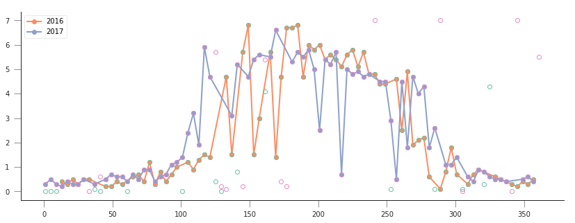
The Nature reserve of Muniellos (43.0156, -6.7038) is mostly populated by Quercus Robur, which shows a strong phenology. It should be a good test point to see whether the data we have is sensible or not.

Using the provided function, plot the time series of LAI over the Muniellos Reserve for 2016 and 2017. Extra points for using QA flags to filter the data

%%html

<div>
     <iframe width="500" height="400" frameborder="0" src="https://www.bing.com/maps/embed?h=400&w=500&cp=43.029897999999996~-6.734863999999996&lvl=11&typ=d&sty=h&src=SHELL&FORM=MBEDV8" scrolling="no">
     </iframe>
     <div style="white-space: nowrap; text-align: center; width: 500px; padding: 6px 0;">
        <a id="largeMapLink" target="_blank" href="https://www.bing.com/maps?cp=43.029897999999996~-6.734863999999996&amp;sty=h&amp;lvl=11&amp;FORM=MBEDLD">View Larger Map</a> &nbsp; | &nbsp;
        <a id="dirMapLink" target="_blank" href="https://www.bing.com/maps/directions?cp=43.029897999999996~-6.734863999999996&amp;sty=h&amp;lvl=11&amp;rtp=~pos.43.029897999999996_-6.734863999999996____&amp;FORM=MBEDLD">Get Directions</a>
    </div>
</div>~

View Larger Map   |   Get Directions

~

y_location, x_location = 43.0156, -6.7038
plt.figure(figsize=(14,5))
for year in [2016, 2017]:
    lai_raster = f"data/euro_lai/Europe_mosaic_Lai_500m_{year:d}.tif"
    qa_raster = f"data/euro_lai/Europe_mosaic_FparLai_QC_{year:d}.tif"

    data = read_tseries(lai_raster, y_location, x_location)
    qa = read_tseries(qa_raster, y_location, x_location)

    qa = get_sfc_qc(qa)
    tx = np.arange(len(qa))*4. + 1
    plt.plot(tx[qa<=1], data[qa<=1]/10., 'o-', label=year)
    plt.plot(tx[qa<=3], data[qa<=3]/10., 'o', mfc="none")
plt.legend(loc="best")

1224 4076
1224 4076
1224 4076
1224 4076

<matplotlib.legend.Legend at 0x7f8ffdbb94e0>

/home/ucfajlg/miniconda3/envs/python3/lib/python3.6/site-packages/matplotlib/font_manager.py:1328: UserWarning: findfont: Font family ['sans-serif'] not found. Falling back to DejaVu Sans
  (prop.get_family(), self.defaultFamily[fontext]))

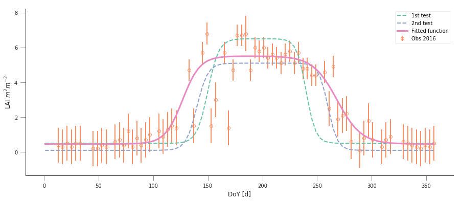
We can now try to fit our double logistic model to the observations, weighted by their uncertainty. We make use the previously defined functions for the model and the cost function that we defined above. We will start by fitting the data to 2016, but will also try to “eyeball” a good starting point for the optimisation. And obviously, we’ll want some plots…

A nice way to plot points with errorbars is (surprisingly enought) the `plt.errorbar method <https://matplotlib.org/api/_as_gen/matplotlib.pyplot.errorbar.html>`__. It’s like the plt.plot method, but it also takes a yerr (or xerr) keyword with the extent of the error in the \(y\) direction.

from scipy.optimize import minimize

plt.figure(figsize=(15, 6))


lat, long = 43.0156, -6.7038
##################################################################
# Start by reading in the data
##################################################################
# Filenames
year = 2016
lai_raster = f"data/euro_lai/Europe_mosaic_Lai_500m_{year:d}.tif"
qa_raster = f"data/euro_lai/Europe_mosaic_FparLai_QC_{year:d}.tif"
# Actually read the data
data = read_tseries(lai_raster, lat, long)/10. # Read LAI
qa = read_tseries(qa_raster, lat, long) # Read QA/QC
# We only want to use QA flags 0 or 1
passer = get_sfc_qc(qa) <= 1
# This is the uncertainty
sigma = get_scaling(get_sfc_qc(qa))[passer]
# This is the time axis: every 4 days
t = np.arange(len(passer))*4 + 1

##################################################################
# Plot the observations of LAI with uncertainty bands
##################################################################

plt.errorbar(t[passer], data[passer], yerr=sigma, fmt="o",
             mfc="none", label=f"Obs {year:d}")

##################################################################
# Plot a first prediction with some random model parameters
##################################################################
# First eyeballing test:
p0 = np.array([0.5, 6, 0.2, 150, 0.23, 240])
plt.plot(t, dbl_sigmoid_function(p0, t), '--', label="1st test")
print("Cost: ",
      cost_function(p0, t, data[passer], passer, sigma))

##################################################################
# Plot a second, more refined prediction
##################################################################

# Second eyeballing test:
p0 = np.array([0.1, 5, 0.2, 140, 0.23, 260])
plt.plot(t, dbl_sigmoid_function(p0, t), '--', label="2nd test")
print("Cost: ",
      cost_function(p0, t, data[passer], passer, sigma))

##################################################################
# Do the minimisation starting from the second prediction
##################################################################

# Now, minimise based on the second test, which appears better

retval2016 = minimize(cost_function, p0, args=(t, data[passer],
                                               passer, sigma))

print(f"Value of the function at the minimum: {retval2016.fun:g}")
print(f"Value of the solution: {str(retval2016.x):s}")

##################################################################
# Plot the fitted model
##################################################################

plt.plot(t, dbl_sigmoid_function(retval2016.x, t), '-', lw=3,
         label="Fitted function")
plt.legend(loc="best")
plt.ylabel("LAI $m^{2}m^{-2}$")
plt.xlabel("DoY [d]")

1224 4076
1224 4076
Cost:  173.30984000080434
Cost:  89.70477658818041
Value of the function at the minimum: 43.7381
Value of the solution: [4.61179375e-01 5.04359058e+00 1.24979192e-01 1.26813991e+02
 9.04932708e-02 2.68361855e+02]

Text(0.5,0,'DoY [d]')

/home/ucfajlg/miniconda3/envs/python3/lib/python3.6/site-packages/matplotlib/font_manager.py:1328: UserWarning: findfont: Font family ['sans-serif'] not found. Falling back to DejaVu Sans
  (prop.get_family(), self.defaultFamily[fontext]))

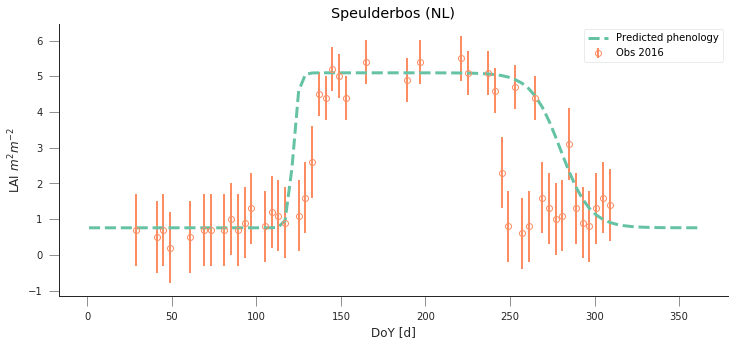
A model isn’t very useful if you can’t use it to make predictions. So let’s just use the optimal solution to predict the LAI for 2017:

plt.figure(figsize=(15, 6))

year = 2017
lai_raster = f"data/euro_lai/Europe_mosaic_Lai_500m_{year:d}.tif"
qa_raster = f"data/euro_lai/Europe_mosaic_FparLai_QC_{year:d}.tif"

data = read_tseries(lai_raster, lat, long)/10. # Read LAI
qa = read_tseries(qa_raster, lat, long) # Read QA/QC
passer = get_sfc_qc(qa) <= 1
sigma = get_scaling(get_sfc_qc(qa))[passer]

t = np.arange(len(passer))*4 + 1

# Plot the data with uncertainty bars
plt.errorbar(t[passer], data[passer], yerr=sigma, fmt="o",
             mfc="none", label=f"Obs {year:d}")

# Print the fitted model
plt.plot(t, dbl_sigmoid_function(retval2016.x, t), '--', lw=3,
         label="Predicted phenology")
plt.legend(loc="best")
plt.ylabel("LAI $m^{2}m^{-2}$")
plt.xlabel("DoY [d]")

1224 4076
1224 4076

Text(0.5,0,'DoY [d]')

/home/ucfajlg/miniconda3/envs/python3/lib/python3.6/site-packages/matplotlib/font_manager.py:1328: UserWarning: findfont: Font family ['sans-serif'] not found. Falling back to DejaVu Sans
  (prop.get_family(), self.defaultFamily[fontext]))

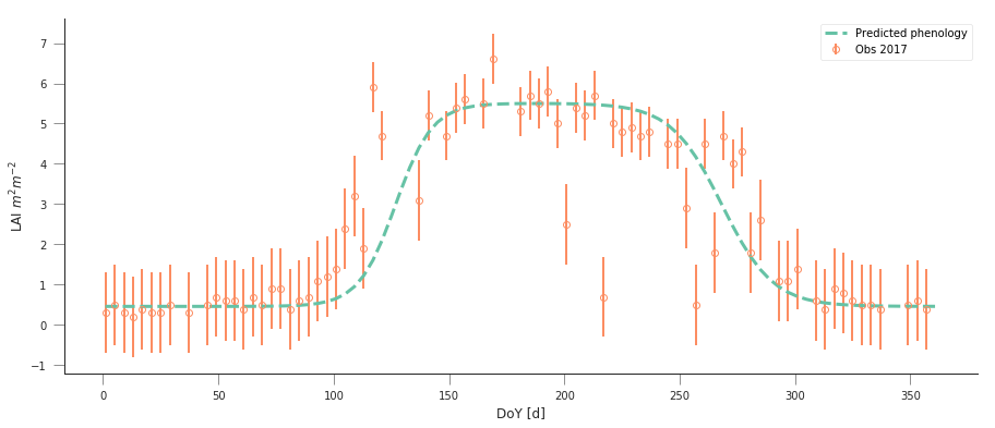
The results are very encouraging, but given the large error bars, and the paucity of data in spring and autumn, can we be sure? We could definitely compare the fit from last year to the fit from this year and see whether they’re different. But it’ll be hard to decide whether they are different or not if we don’t have error bars in the parameters!

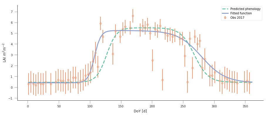
Fit the phenology model to the 2017 data, and comment on the optimal parameters

plt.figure(figsize=(15, 6))

year = 2017
lai_raster = f"data/euro_lai/Europe_mosaic_Lai_500m_{year:d}.tif"
qa_raster = f"data/euro_lai/Europe_mosaic_FparLai_QC_{year:d}.tif"

data = read_tseries(lai_raster, lat, long)/10. # Read LAI
qa = read_tseries(qa_raster, lat, long) # Read QA/QC
passer = get_sfc_qc(qa) <= 1
sigma = get_scaling(get_sfc_qc(qa))[passer]

t = np.arange(len(passer))*4 + 1

# Plot the data with uncertainty bars
plt.errorbar(t[passer], data[passer], yerr=sigma, fmt="o",
             mfc="none", label=f"Obs {year:d}")

# Print the fitted model
plt.plot(t, dbl_sigmoid_function(retval2016.x, t), '--', lw=3,
         label="Predicted phenology")
print(f"Value from previous year: {str(retval2016.x):s}")
retval2017 = minimize(cost_function, p0, args=(t, data[passer], passer,
                                                 sigma))


print(f"Value of the function at the minimum: {retval2017.fun:g}")
print(f"Value of the solution: {str(retval2017.x):s}")


# Print the fitted model
plt.plot(t, dbl_sigmoid_function(retval2017.x, t), '-', lw=3,
         label="Fitted function")

plt.legend(loc="best")
plt.ylabel("LAI $m^{2}m^{-2}$")
plt.xlabel("DoY [d]")

1224 4076
1224 4076
Value from previous year: [4.61179375e-01 5.04359058e+00 1.24979192e-01 1.26813991e+02
 9.04932708e-02 2.68361855e+02]
Value of the function at the minimum: 41.6294
Value of the solution: [4.17809359e-01 4.83020921e+00 1.97608815e-01 1.07388496e+02
 5.23646758e-02 2.79806238e+02]

Text(0.5,0,'DoY [d]')

/home/ucfajlg/miniconda3/envs/python3/lib/python3.6/site-packages/matplotlib/font_manager.py:1328: UserWarning: findfont: Font family ['sans-serif'] not found. Falling back to DejaVu Sans
  (prop.get_family(), self.defaultFamily[fontext]))

Do a similar experiment for other sites. In the benefit of efficiency, you could write a set of functions that would allow you to quickly do the entire process and relevant plots for different latitude/longitude points

Some quick notions on how to develop the functions:

1. You probably want a read data function, that returns LAI, sigma and passer.

2. A second function could take the data and a starting guess, and minimise it, returning the optimal parameters.

3. A third function would be in charge of plotting the data, and the predictions, so it could take the observations and uncertainties, etc., as well as a vector of parameters.

4. A final function could wrap the previous three and allow the user to select a year to fit to and a location

You can probably come up with interesting sites, but here are some that you may want to try

sites = [[43.015364, -6.703704],
         [51.775511, -1.336993],
         [43.487178, 1.283292]
        ]

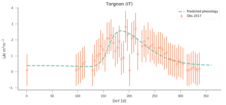
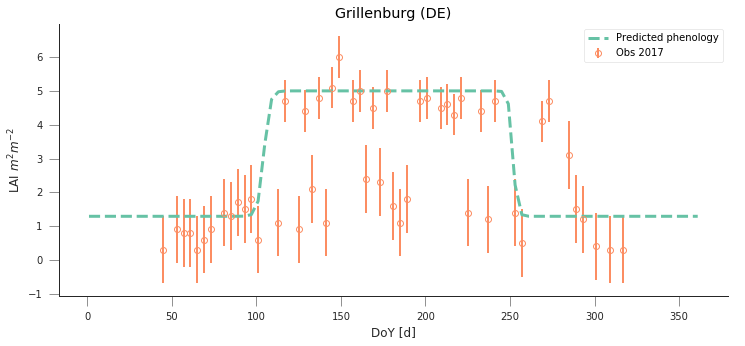
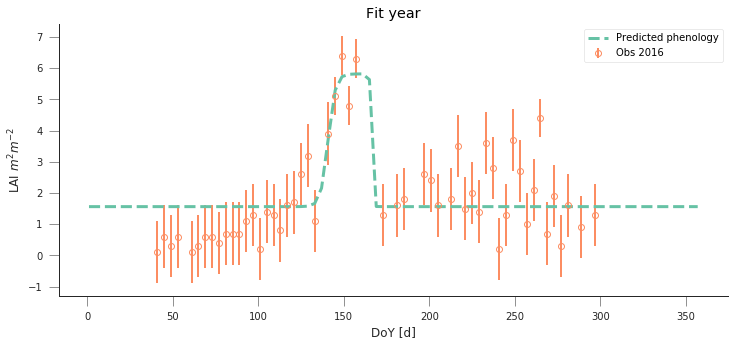
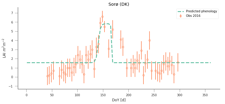
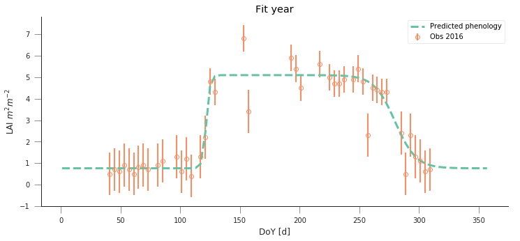
I have fished out some suitable location from the paper from Wingate et al (2015), and you can see the results of fitting to the model to (some of) the sites below:

def read_data(year, x_location, y_location):
    """A function to read in data from the given LAI and QC maps. The
    function also converts the QA data into a `passer` (on/off) array
    to filter the really bad observations, and also creates `sigma`,
    the pseudo-uncertainty.

    Parameters
    -----------
    x_location: float
        The longitude in decimal degrees.
    y_location: float
        The latitude in decimal degrees.

    Returns
    --------

    A time arrray, the data (LAI, scaled properly), the uncertainty and the
    `passer` mask
    """
    lai_raster = f"data/euro_lai/Europe_mosaic_Lai_500m_{year:d}.tif"
    qa_raster = f"data/euro_lai/Europe_mosaic_FparLai_QC_{year:d}.tif"
    print(lai_raster)
    data = read_tseries(lai_raster, y_location, x_location)/10.
    qa = read_tseries(qa_raster, y_location, x_location)
    passer = get_sfc_qc(qa) <= 1
    sigma = get_scaling(get_sfc_qc(qa))[passer]

    t = np.arange(len(passer))*4 + 1
    return t, data, sigma, passer

def fit_data(t, data, sigma, passer,
            cost_f=cost_function,
            p0= np.array([0.1, 5, 0.2, 140, 0.23, 260])):
    """Fits the data using scipy.optimize `minimize` function. It's a wrapper
    around a cost function given by `cost_f` (by default, it)"""
    retval = minimize(cost_f, p0, args=(t, data[passer], passer, sigma))
    return retval

def do_plots(t, data, sigma, passer, p):
    """Do some plots"""

    # Plot the data with uncertainty bars
    plt.errorbar(t[passer], data[passer], yerr=sigma, fmt="o",
             mfc="none", label=f"Obs {year:d}")
    # Print the fitted model
    plt.plot(t, dbl_sigmoid_function(p, t), '--', lw=3,
         label="Predicted phenology")
    plt.legend(loc="best")
    plt.ylabel("LAI $m^{2}m^{-2}$")
    plt.xlabel("DoY [d]")

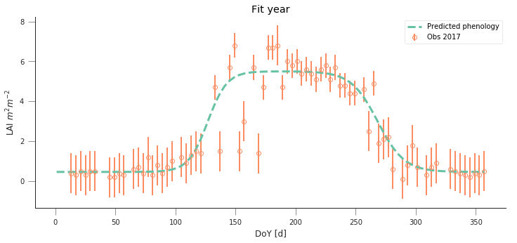
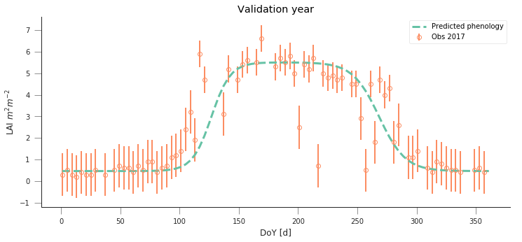
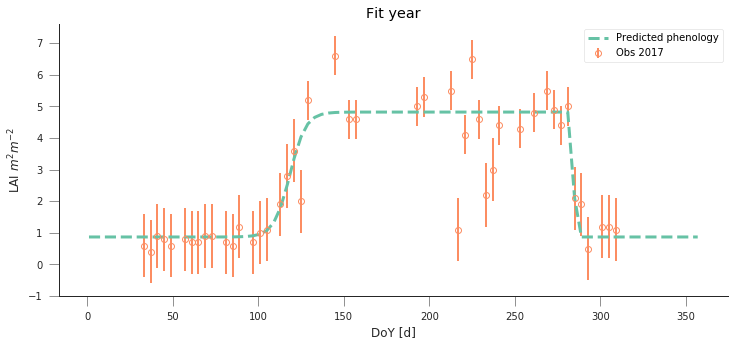
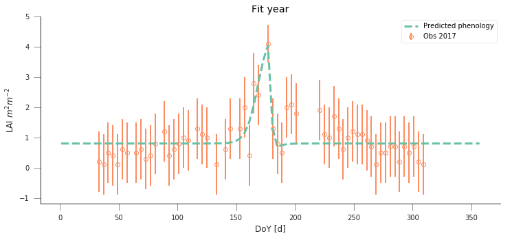
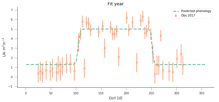
def fit_data_year(fit_year, val_year, x_location, y_location):
    plt.figure(figsize=(12, 5))
    t, data, sigma, passer = read_data(fit_year, x_location,
                                       y_location)
    optimal_p = fit_data(t, data, sigma, passer)
    do_plots(t, data, sigma, passer, optimal_p.x)
    t, data, sigma, passer = read_data(val_year, x_location,
                                       y_location)
    plt.title("Fit year")
    plt.figure(figsize=(12, 5))
    do_plots(t, data, sigma, passer, optimal_p.x)
    plt.title("Validation year")


fit_data_year(2016, 2017, x_location, y_location)

data/euro_lai/Europe_mosaic_Lai_500m_2016.tif
1224 4076
1224 4076
data/euro_lai/Europe_mosaic_Lai_500m_2017.tif
1224 4076
1224 4076

/home/ucfajlg/miniconda3/envs/python3/lib/python3.6/site-packages/matplotlib/font_manager.py:1328: UserWarning: findfont: Font family ['sans-serif'] not found. Falling back to DejaVu Sans
  (prop.get_family(), self.defaultFamily[fontext]))

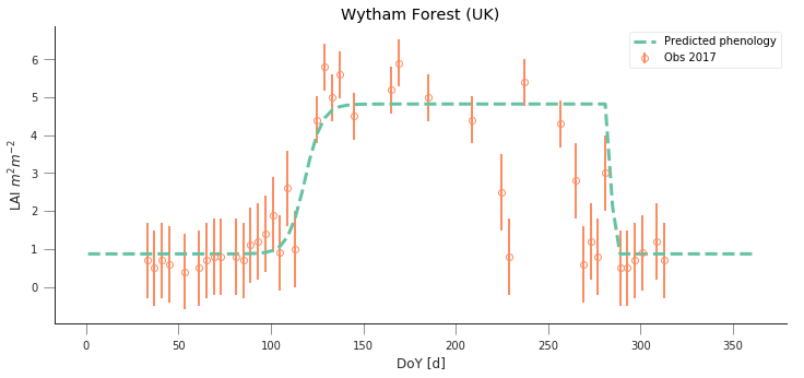
y_location, x_location = 51.775511, -1.336993
fit_data_year(2016, 2017, x_location, y_location)
plt.title("Wytham Forest (UK)")

data/euro_lai/Europe_mosaic_Lai_500m_2016.tif
2201 1974
2201 1974
data/euro_lai/Europe_mosaic_Lai_500m_2017.tif
2201 1974
2201 1974

Text(0.5,1,'Wytham Forest (UK)')

/home/ucfajlg/miniconda3/envs/python3/lib/python3.6/site-packages/matplotlib/font_manager.py:1328: UserWarning: findfont: Font family ['sans-serif'] not found. Falling back to DejaVu Sans
  (prop.get_family(), self.defaultFamily[fontext]))

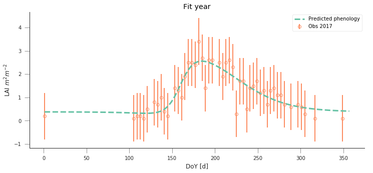
y_location, x_location = 45.8444, 7.5781
fit_data_year(2016, 2017, x_location, y_location)
plt.title("Torgnon (IT)")

data/euro_lai/Europe_mosaic_Lai_500m_2016.tif
3667 3397
3667 3397
data/euro_lai/Europe_mosaic_Lai_500m_2017.tif
3667 3397
3667 3397

Text(0.5,1,'Torgnon (IT)')

/home/ucfajlg/miniconda3/envs/python3/lib/python3.6/site-packages/matplotlib/font_manager.py:1328: UserWarning: findfont: Font family ['sans-serif'] not found. Falling back to DejaVu Sans
  (prop.get_family(), self.defaultFamily[fontext]))

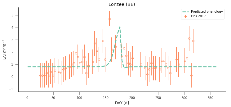
y_location, x_location = 50.5516, 4.7461
fit_data_year(2016, 2017, x_location, y_location)
plt.title("Lonzee (BE)")

data/euro_lai/Europe_mosaic_Lai_500m_2016.tif
3124 2268
3124 2268
data/euro_lai/Europe_mosaic_Lai_500m_2017.tif
3124 2268
3124 2268

Text(0.5,1,'Lonzee (BE)')

/home/ucfajlg/miniconda3/envs/python3/lib/python3.6/site-packages/matplotlib/font_manager.py:1328: UserWarning: findfont: Font family ['sans-serif'] not found. Falling back to DejaVu Sans
  (prop.get_family(), self.defaultFamily[fontext]))

y_location, x_location = 50.9500, 13.5126
fit_data_year(2016, 2017, x_location, y_location)
plt.title("Grillenburg (DE)")

data/euro_lai/Europe_mosaic_Lai_500m_2016.tif
4443 2172
4443 2172
data/euro_lai/Europe_mosaic_Lai_500m_2017.tif
4443 2172
4443 2172

Text(0.5,1,'Grillenburg (DE)')

/home/ucfajlg/miniconda3/envs/python3/lib/python3.6/site-packages/matplotlib/font_manager.py:1328: UserWarning: findfont: Font family ['sans-serif'] not found. Falling back to DejaVu Sans
  (prop.get_family(), self.defaultFamily[fontext]))

y_location, x_location = 55.4859,11.6446
fit_data_year(2016, 2017, x_location, y_location)
plt.title("Sorø (DK)")

data/euro_lai/Europe_mosaic_Lai_500m_2016.tif
3984 1083
3984 1083
data/euro_lai/Europe_mosaic_Lai_500m_2017.tif
3984 1083
3984 1083

Text(0.5,1,'Sorø (DK)')

/home/ucfajlg/miniconda3/envs/python3/lib/python3.6/site-packages/matplotlib/font_manager.py:1328: UserWarning: findfont: Font family ['sans-serif'] not found. Falling back to DejaVu Sans
  (prop.get_family(), self.defaultFamily[fontext]))

y_location, x_location =52.253000000000, 5.702000000000

fit_data_year(2016, 2017, x_location, y_location)
plt.title("Speulderbos (NL)")

data/euro_lai/Europe_mosaic_Lai_500m_2016.tif
3238 1859
3238 1859
data/euro_lai/Europe_mosaic_Lai_500m_2017.tif
3238 1859
3238 1859

Text(0.5,1,'Speulderbos (NL)')

/home/ucfajlg/miniconda3/envs/python3/lib/python3.6/site-packages/matplotlib/font_manager.py:1328: UserWarning: findfont: Font family ['sans-serif'] not found. Falling back to DejaVu Sans
  (prop.get_family(), self.defaultFamily[fontext]))

Uncertainty

In the previous examples, we have seen that the model can be made to fit observations and used in prediction pretty well, but there’s the obvious question of how exactly can we define the different parameters. Ideally, we’d like to have some error bars on e.g. the date and slope of the spring and autumn flanks, so that we can decide whether a shift has ocurred or not. Similarly for the maximum/minimum LAI. Intuitively, we can see that if we change the optimal parameters a bit, we’ll get a solution that might still have an acceptable performance (meaning that it will probably go through all the error bars).

One way to test this is to do some Monte Carlo sampling around the optimal solution. We can evaluate the shape of the cost function around the optimum and that will give us an idea of the uncertainty: a cost function that changes very rapidly around the optimal point in one direction suggests that if you change the parameters by a small amount, the goodness of fit changes drastically, so that the parameter is very well and accurately defined. In contrast, if changing the parameter doesn’t change the cost function value by much, we have an uncertain parameter.

The Metropolis-Hastings algorithm

A way to do this Monte Carlo sampling is to use the Metropolis-Hastings algorithm. This is a sequential method that proposes and accepts samples based on the likelihood value. Basically, if the cost function improves, the sample gets accepted, if it doesn’t improve, then a uniform random number between 0 and 1 is drawn. If the ratio of proposed to previous likelihoods is greater than the random number, the samples gets accepted. This means that for solutions that don’t improve the cost function, there’s a chance that the algorithm will improve on them, meaning that it doesn’t get trapped on local minima, and provides an exploration of the entire problem space.

In a nutshell, here’s some pseudocode of the MH algorithm

1. Initialise \(\vec{x}^{0}\).
2. For \(i=1\) to \(i=N_{iterations}\):
   1. Sample a proposed new \(\vec{x}^{*}\) as \(\vec{x}^{*}=\vec{x}^{i-1} + \mathcal{N}(0, \Sigma)\).
   2. Calculate the likelihood associated with \(\vec{x}^{*}\), \(L(\vec{x}^{*}, i)\).
   3. Calculate the likelihood ratio \(\alpha=\displaystyle{\frac{L(\vec{x}^{*}, i)}{L(\vec{x}^{*}, i-1)}}\).
   4. Draw a random uniform number between 0 and 1 \(u=\mathcal{U}(0,1)\)
   5. if \(u\le \min\left\lbrace 1, \alpha\right\rbrace\):
   6. \(\vec{x}^{i+1} = \vec{x}^{*}\): we accept the new proposal
   7. else:
   8. \(\vec{x}^{i+1} = \vec{x}^{i}\): we reject the new proposal

Examine the MH algorithm, and try to see whether you can see how you could go and implement it in Python. The pseudocode above presents you with the barebones recipe, and you will need to add a couple of extra ingredients. You can assume that you have available the log-likelihood function that we have described above, and you may need to use the np.random.normal and np.random.rand functions which respectively provide Gaussian random numbers and uniform random numbers between 0 and 1

def metropolis_hastings(xstart, lklhood, year, x_location, y_location,
                        n_iter=50000):
    """MH algorithm implementation. Takes a starting vector, a log-likelihood
    function, a year and an x and y location (in degrees), as well as a number
    of iterations. We are assuming that a `read_data` function that will read
    data and return a time axis, the LAI, the uncertainties and a mask object
    is available. We also assume that the lklhood function can be called using
    these data as `(x_proposed, t, data[passer], passer,sigma)`
    """
    # We first read in the data. this only happens once
    t, data, sigma, passer = read_data(year, x_location, y_location)
    n_params = len(xstart)
    # We reserve some storage for the posterior samples
    samples = np.zeros((n_iter, n_params))
    # We start. Set up xstart as our current parameter vector
    x_curr = xstart*1.
    # Calculate the initial cost function/log-likelihood
    old_cost = lklhood(x_curr, t, data[passer], passer,
                                sigma)
    # Now iterate...
    for i in range(n_iter):
        # Random displacement
        x_proposed = x_curr + np.random.normal(
            size=n_params)*np.array([0.1,
                                     0.1,
                                     0.01,
                                     5.,
                                     0.01,
                                     5])
        # Now, calculate the cost function for the proposed parameter
        # vector...
        proposed_cost = lklhood(x_proposed, t, data[passer], passer,
                                sigma)
        # This is the Metropolis acceptance: if the proposed cost is greater
        # than the previous one, accept, if not sometimes accept
        if np.random.rand() < np.exp(proposed_cost - old_cost):
            # We have accepted the proposed parameter. We update x_curr
            # to match, and updated proposed_cost to the current cost
            x_curr = x_proposed
            old_cost = proposed_cost
        # if we don't accept (because the proposed cost is less, and the
        # difference is below the random draw) we keep the old cost, and
        # do not update x_curr
        # We store the samples nevertheless!!
        samples[i, :] = x_proposed

    return samples

y_location, x_location = 43.0156, -6.7038

def read_data(year, x_location, y_location):
    lai_raster = f"data/euro_lai/Europe_mosaic_Lai_500m_{year:d}.tif"
    qa_raster = f"data/euro_lai/Europe_mosaic_FparLai_QC_{year:d}.tif"
    print(lai_raster)
    data = read_tseries(lai_raster, y_location, x_location)/10.
    qa = read_tseries(qa_raster, y_location, x_location)
    passer = get_sfc_qc(qa) <= 1
    sigma = get_scaling(get_sfc_qc(qa))[passer]

    t = np.arange(len(passer))*4 + 1
    return t, data, sigma, passer

def lklhood(p, t, y_obs, passer, sigma_obs, func=dbl_sigmoid_function):
    y_pred = func(p, t)
    n = passer.sum()
    cost = -0.5* (y_pred[passer]-y_obs)**2/sigma_obs**2
    return cost.sum()




samples = metropolis_hastings(retval2016.x, lklhood,
                              2016, x_location, y_location,
                             n_iter=100000)

data/euro_lai/Europe_mosaic_Lai_500m_2016.tif
1224 4076
1224 4076

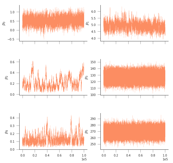
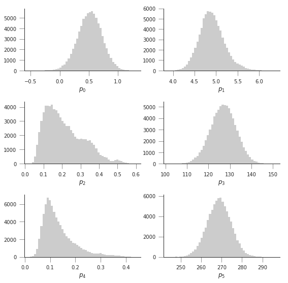
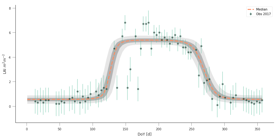
The previous code has produced samples of parameters that we can now visualise as “traces” as well as histograms. The shape of the histograms gives us some idea of the uncertainty of the parameters in their units. We can also use these samples and propagate them through the phenology model to produce an ensemble of model trajectories that define a region of uncertainty.

fig, axs = plt.subplots(nrows=3, ncols=2, figsize=(9, 9), sharex=True)
axs = axs.flatten()
for i in range(len(retval2016.x)):
    axs[i].plot(samples[:, i], '-', lw=0.2)
    axs[i].set_ylabel(f"$p_{i}$")

fig, axs = plt.subplots(nrows=3, ncols=2, figsize=(9, 9))
axs = axs.flatten()
for i in range(len(retval2016.x)):
    axs[i].hist(samples[20000:, i], bins=50, color="0.8")
    axs[i].set_xlabel(f"$p_{i}$")

/home/ucfajlg/miniconda3/envs/python3/lib/python3.6/site-packages/matplotlib/font_manager.py:1328: UserWarning: findfont: Font family ['sans-serif'] not found. Falling back to DejaVu Sans
  (prop.get_family(), self.defaultFamily[fontext]))

n_samples = samples.shape[0]
y_location, x_location = 43.0156, -6.7038

t, data, sigma, passer = read_data(2016, x_location, y_location)

pred_lai = np.zeros((n_samples, len(t)))
for i in range(n_samples):
    pred_lai[i, :] = dbl_sigmoid_function(samples[i], t)


plt.figure(figsize=(15, 7))
pcntiles = np.percentile( pred_lai[60000::20], [5, 25, 50, 75, 95], axis=0)
plt.fill_between(t, pcntiles[0], pcntiles[-1], color="0.9")
plt.fill_between(t, pcntiles[1], pcntiles[-2], color="0.7")
plt.plot(t, pcntiles[2], '--', lw=3, label="Median")

plt.errorbar(t[passer], data[passer], yerr=sigma, fmt="o",
             mfc="none", label=f"Obs {year:d}", alpha=0.5)

plt.legend(loc="best")
plt.ylabel("LAI $m^{2}m^{-2}$")
plt.xlabel("DoY [d]")

data/euro_lai/Europe_mosaic_Lai_500m_2016.tif
1224 4076
1224 4076

Text(0.5,0,'DoY [d]')

/home/ucfajlg/miniconda3/envs/python3/lib/python3.6/site-packages/matplotlib/font_manager.py:1328: UserWarning: findfont: Font family ['sans-serif'] not found. Falling back to DejaVu Sans
  (prop.get_family(), self.defaultFamily[fontext]))

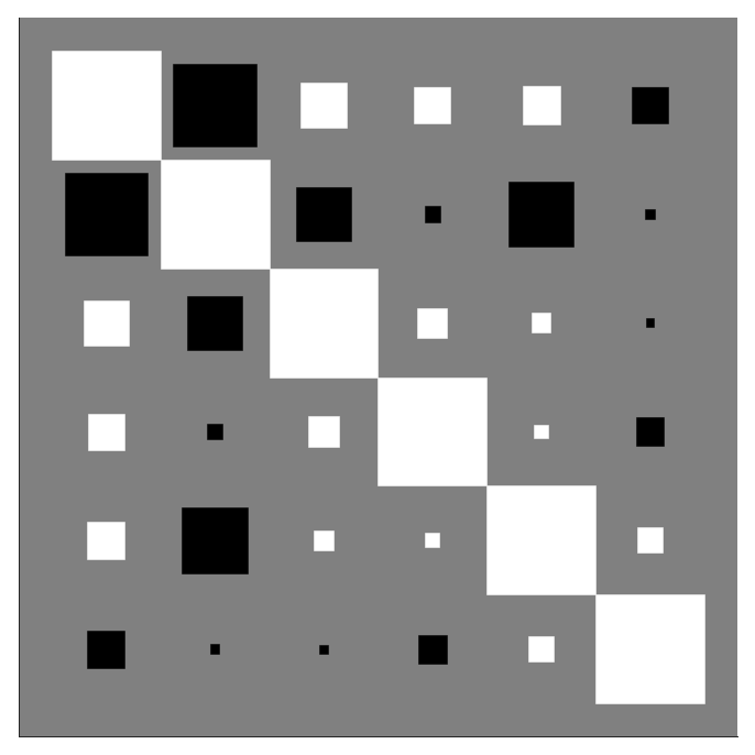
cov = np.corrcoef(samples[60000::20, :].T)

def hinton(matrix, max_weight=None, ax=None):
    """Draw Hinton diagram for visualizing a weight matrix."""
    ax = ax if ax is not None else plt.gca()

    if not max_weight:
        max_weight = 2 ** np.ceil(np.log(np.abs(matrix).max()) / np.log(2))

    ax.patch.set_facecolor('gray')
    ax.set_aspect('equal', 'box')
    ax.xaxis.set_major_locator(plt.NullLocator())
    ax.yaxis.set_major_locator(plt.NullLocator())

    for (x, y), w in np.ndenumerate(matrix):
        color = 'white' if w > 0 else 'black'
        size = np.sqrt(np.abs(w) / max_weight)
        rect = plt.Rectangle([x - size / 2, y - size / 2], size, size,
                             facecolor=color, edgecolor=color)
        ax.add_patch(rect)

    ax.autoscale_view()
    ax.invert_yaxis()

plt.figure(figsize=(12,12))
hinton(cov)