Table of Contents

• 4. Assessed Practical

  • 4.1 Introduction

    • 4.1.1 Task overview

  • 4.1.2 Purpose of the work

    • 4.2.1.1 Del Norte

    • 4.2.1.2 Discharge dataset

    • 4.2.1.3 Temperature dataset

    • 4.2.1.4 Snow cover dataset

    • 4.2.2 Data Advice

      • 4.2.2.1 MODIS snow cover data

      • 4.2.3.2 Boundary Data

      • 4.2.3.3 Discharge Data

      • 4.2.3.4 Temperature data

  • 4.3 Coursework

    • 6.3.1 Summary of coursework requirements

    • 4.3.2 Summary of Advice

    • 4.3.3 Further advice

    • 4.3.4 Structure of the Report

    • 4.3.5 Computer Code

      • General requirements

      • Degree of original work required and plagiarism

      • Documentation

      • Word limit

      • Code style

4. Assessed Practical

4.1 Introduction

4.1.1 Task overview

These notes describe the practical work you must submit for assessment in this course.

The practical comes in two parts: (1) data preparation (50%); (2) modelling (50%).

It is important that you complete both parts of this exercise.

The submission for Part 1 of the coursework (worth 50% of the marks) is the Monday after Reading week (12:00 Noon). That is Monday \(12^{th}\) November 2018.

The submission for Part 2 will be \(7^{th}\) January 2019 (12:00 Noon). Submission is through the usual Turnitin link on the course Moodle page.

• Part 1: Data Preparation

  The first task you must complete is to produce a dataset of the proportion of HUC catchment 13010001 (Rio Grande headwaters in Colorado, USA) that is covered by snow for two years (not necessarily consecutive), along with associated datasets on temperature (in C) and river discharge at the Del Norte monitoring station. You will use these data in the modelling work in Part 2 of the coursework.

  You may not use data from the years 2005 or 2006, as this will be given to you in illustrations of the material.

  The dataset you produce must have a value for the mean snow cover, temperature and discharge in the catchment for every day over each year.

  Your write up must include fully labelled graph(s) of snow cover, temperature and discharge for the catchment for each year (with units as appropriate), along with some summary statistics (e.g. mean or median, minimum, maximum, and the timing of these).

  You must provide evidence of how you got these data (i.e. the code and commands you ran to produce the data).

Checklist:

* provide fully commented/documented code for all operations.
* provide two years of **daily** data (not 2005 or 2006)
* Generate datasets of:
    * mean snow cover (0.0 to 1.0) for the catchment for each day of the year
    * temperature (C) at the Del Norte monitoring station for each day of the year
    * river discharge at the Del Norte monitoring station for each day of the year
* Produce a table of summary statistics for each of the 3 datasets (one for easch year)
* produce graphs of the 3 datasets for each year (as function of day of year)
* produce an `npz` file containing the 3 datasets, one for each year.
* produce images of snow cover spatial data for the catchment for **13 samples** spaced equally through the year, one set of images for each year. You need to do this for the data pre-interpolation and aftyer you have done the interpolation.

• Part 2: Modelling

  You will have prepared two years of data in Part 1 of the work.

  If, for some reason, you have failed to generate an appropriate dataset, you may use datasets that will be provided for you for the years 2005 and 2006. There will be no penalty for that in your Part 2 submission: failure to gernerate the datasets will be accounted for in marks allocated for Part 1.

  You will be given a simple hydrological model of snowmelt.

  Use one of these years to calibrate the (snowmelt) hydrological model and one year to test it.

  The model parameter estimate must be objective (i.e. you can’t just arbitrarily choose a set) and optimal in some way you must define (you must state the equation of the cost function you will try to minimise and explain the approach used).

  You must state the values of the model parameters that you have estimated and show evidence for how you went about calculating them. Ideally, you should also state the uncertainty in these parameter estimates (not critical to pass this section though).

  You must quantify the goodness of fit between your measured flow data and that produced by your model, both for the calibration exercise and the validation.

Checklist:

* Provide a site intoduction and an introduction to the purpose of the exercise ('Introduction')
* Provide an introduction to the modelling and calibration/validation ('Method')
* provide code that reads in the datasets and performs the model calibration and validation ('Code')
* Provide a table of results on model parameter calibration (and ideally, uncertainty) ('Results')
* Provide graphs of the observed and modelled river discharge data for the calibration year ('Results')
* Provide graphs of the observed and modelled river discharge data for the validation year ('Results')
* Assess the accuracy of the calibration and validation ('Results')
* Discuss the results in the light of the introduction ('Discussion')
* Draw conclusions about issues associated with modelling of this sort ('Conclusion')

You must work individually on this task. If you do not, it will be treated as plagiarism. By reading these instructions for this exercise, we assume that you are aware of the UCL rules on plagiarism. You can find more information on this matter in your student handbook. If in doubt about what might constitute plagiarism, ask one of the course convenors.

4.1.2 Purpose of the work

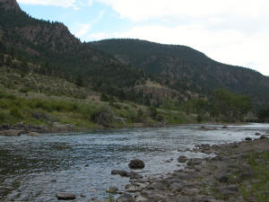
The hydrology of the Rio Grande Headwaters in Colorado, USA is snowmelt dominated. It varies considerably from year to year and may very further under a changing climate.

We can build a mathemetical (‘environmental’) model to describe the main physical processes affecting hydrology in the catchment. Such a model could help understand current behaviour and allow some prediction about possible future scenarios.

What you are going to do is to build, calibrate and test a (snowmelt) hydrological model, driven by observations in the Rio Grande Headwaters in Colorado, USA

The purpose of the model will be to describe the streamflow at the Del Norte measurement station, just on the edge of the catchment. You will use environmental (temperature) data and snow cover observations to drive the model. You will perform calibration and testing by comparing model output with observed streamflow data.

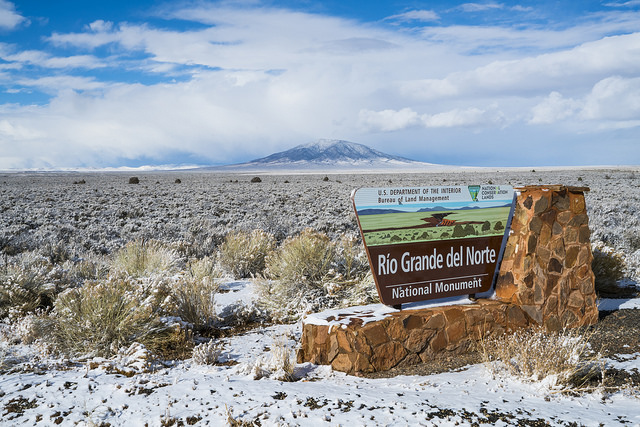
4.2.1.1 Del Norte

The average climate for Del Norte is:

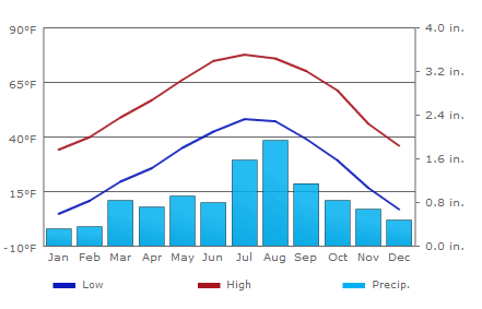
Further general information is available from various websites, including NOAA.

www.coloradofishing.net

You can visualise the site Del Norte 2E here.

4.2.1.2 Discharge dataset

First we should look at the streamflow/discharge data.

The link for downloading data from 2001 onwards (but not the current year until the end of the year): http://waterdata.usgs.gov.

You should examine all of the streamflow data and use that to make a decision on which years data you want to use in your experiments. You must justify your decision. You choice coul;d be based on the fact that some particular year shows ‘typical’ behaviour, or that some set of years seems to encompass the bounds of behaviour. The choies you make here will impact your ability to generalise from your results, so make sure you comment on this.

write some code to download the data, select one of the years that you want, and load the data into numpy arrays of time and streamflow (discharge).

run the code for the two years of data that you have selected and save the datasets to a file.

4.2.1.3 Temperature dataset

Go to the Colorado State Climate data site, select the Del Norte 2E site, and the period for which you want your data (typically, Jan \(1^{st}\) to Dec \(31^{st}\) for the years you want.

You can obtain data on maximum and mimimum temperatures, as well as snowfall and precipitation.

As the site doesn’t provide a data download mechanism, you will need to save the data, most easily by copying and pasting the data columns into a file. Make a note of what you did here, to include in your write up.

You only really need the maximum temperature dataset, but you may find the others helpful for interpretation or to improve your model.

4.2.1.4 Snow cover dataset

You need to calculate the daily snow cover (values between 0 and 1 for the proportion of the catchment covered in snow) for the catchment (HUC feature 2 (catchment 13010001)).

You would want to use a daily snow product for this task, such as that available from MODIS, so make sure you know what that is and explore the characteristics of the dataset.

You will notice from the figure above (the figure should give you some clue as to a suitable data product) that there will be areas of each image for which you have no information (described in the dataset QC). You will need to decide what to do about ‘missing data’. For instance, you might consider interpolating over missing values.

The simplest thing you might think of might be to produce a mean snow cover over what samples are available (ignoring the missing values). But that would be rather poor. Really, you should apply some sort of interpolation (in time).

However you decide to process the data, you must give a rationale for why you have taken the approach you have done.

You will notice that if you use MODIS data, you have access to both data from Terra (MOD10A) and Aqua (MYD10A), which potentially gives you two samples per day. Think about how to take that into account. Again, the simplest thing to do might be to just use one of these. That is likely to be sufficient, but it would be much better to include both datasets.

# load a pre-cooked version of the data for 2005 (NB -- Dont use this year!!!
# except perhaps for testing)

# load the data from a pickle file
import pickle
import pylab as plt
import numpy as np
%matplotlib inline

with open('data/data.pkl', 'rb') as f:
    data = pickle.load(f, encoding='latin1')

# set up plot
plt.figure(figsize=(10,5))
plt.xlim(data['doy'][0],data['doy'][-1]+1)
plt.xlabel('day of year 2005')

# plot data
plt.plot(data['doy'],data['temp'],'r',label='temperature / C')
plt.plot(data['doy'],data['snowprop']*100,'b',label='snow cover %')
plt.plot(data['doy'],100-data['snowprop']*100,'c',label='snow free cover %')
plt.plot(data['doy'],data['flow']/100.,'g',label='river flow / 100')
plt.legend(loc='best')

<matplotlib.legend.Legend at 0x10725edd8>

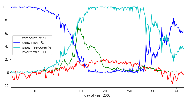
we have plotted the streamflow (scaled) in green, the snow cover in blue, and the non snow cover in cyan and the temperature in red. It should be apparent that thge hydrology is snow melt dominated, and to describe this (i.e. to build the simplest possible model) we can probably just apply some time lag function to the snow cover.

4.2.2 Data Advice

4.2.2.1 MODIS snow cover data

For MODIS data, you will need to work out which data product you want and how to download it. To help you with this, the ‘pattern’ of the URLs is:

info = {'YEAR':2007,'MONTH':1,'DAY':1}
url = 'https://n5eil01u.ecs.nsidc.org/MOST/MOD10A1.006/' + \
    '{YEAR}.{MONTH:02d}.DAY:02d}/MYD*h09v05.006*hdf'.format(**info)

You should have codes from previous practicals sessions that allow you to download such data and you should then store the daily datasets in you local file system.

We can use the usual tools to explore the MODIS hdf files:

import gdal
modis_file = 'data/MOD10A1.A2016001.h09v05.006.2016183123533.hdf'
g = gdal.Open(modis_file)
if g is None:
    print ('error opening file: HDF4 problem with GDAL?')
else:
    # note this has changed in collection 6
    data_layer = 'MOD_Grid_Snow_500m:NDSI_Snow_Cover'

    subdatasets = g.GetSubDatasets()
    for fname, name in subdatasets:
        print (name)
        print ("\t", fname)

    fname = 'HDF4_EOS:EOS_GRID:"%s":%s'%(modis_file,data_layer)
    raster = gdal.Open(fname)

[2400x2400] NDSI_Snow_Cover MOD_Grid_Snow_500m (8-bit unsigned integer)
     HDF4_EOS:EOS_GRID:"data/MOD10A1.A2016001.h09v05.006.2016183123533.hdf":MOD_Grid_Snow_500m:NDSI_Snow_Cover
[2400x2400] NDSI_Snow_Cover_Basic_QA MOD_Grid_Snow_500m (8-bit unsigned integer)
     HDF4_EOS:EOS_GRID:"data/MOD10A1.A2016001.h09v05.006.2016183123533.hdf":MOD_Grid_Snow_500m:NDSI_Snow_Cover_Basic_QA
[2400x2400] NDSI_Snow_Cover_Algorithm_Flags_QA MOD_Grid_Snow_500m (8-bit unsigned integer)
     HDF4_EOS:EOS_GRID:"data/MOD10A1.A2016001.h09v05.006.2016183123533.hdf":MOD_Grid_Snow_500m:NDSI_Snow_Cover_Algorithm_Flags_QA
[2400x2400] NDSI MOD_Grid_Snow_500m (16-bit integer)
     HDF4_EOS:EOS_GRID:"data/MOD10A1.A2016001.h09v05.006.2016183123533.hdf":MOD_Grid_Snow_500m:NDSI
[2400x2400] Snow_Albedo_Daily_Tile MOD_Grid_Snow_500m (8-bit unsigned integer)
     HDF4_EOS:EOS_GRID:"data/MOD10A1.A2016001.h09v05.006.2016183123533.hdf":MOD_Grid_Snow_500m:Snow_Albedo_Daily_Tile
[2400x2400] orbit_pnt MOD_Grid_Snow_500m (8-bit integer)
     HDF4_EOS:EOS_GRID:"data/MOD10A1.A2016001.h09v05.006.2016183123533.hdf":MOD_Grid_Snow_500m:orbit_pnt
[2400x2400] granule_pnt MOD_Grid_Snow_500m (8-bit unsigned integer)
     HDF4_EOS:EOS_GRID:"data/MOD10A1.A2016001.h09v05.006.2016183123533.hdf":MOD_Grid_Snow_500m:granule_pnt

4.2.3.2 Boundary Data

Boundary data, such as catchments, might typically come as ESRI shapefiles or may be in other vector formats. There tends to be variable quality among different databases, but a reliable source for catchment data the USA is the USGS. One set of catchments in the tile we have is the Rio Grande headwaters, which we can see has a HUC 8-digit code of 13010001. The full dataset is easily found from the USGS or locally. Literature and associated data concerning this area can be found here. Associated GIS data are here, including the watershed boundary data.

Data more specific to our particular catchment of interest can be found on the Rio Grande Data Project pages.

You should use the file Hydrologic_Units.zip. You may need to unzip this file to get at the shapefile `Hydrologic_Units/HUC_Polygons.shp <data/Hydrologic_Units/HUC_Polygons.shp>`__ within it.

You can explore the shape file with the following:

!ogrinfo data/Hydrological_Units/HUC_Polygons.shp HUC_Polygons -nomd -geom=NO -where "HUC=13010001"

INFO: Open of `data/Hydrological_Units/HUC_Polygons.shp'
      using driver `ESRI Shapefile' successful.

Layer name: HUC_Polygons
Geometry: Polygon
Feature Count: 1
Extent: (-1207861.193700, -1295788.385400) - (-115932.919500, 152769.254400)
Layer SRS WKT:
PROJCS["USA_Contiguous_Albers_Equal_Area_Conic",
    GEOGCS["GCS_North_American_1983",
        DATUM["North_American_Datum_1983",
            SPHEROID["GRS_1980",6378137.0,298.257222101]],
        PRIMEM["Greenwich",0.0],
        UNIT["Degree",0.0174532925199433],
        AUTHORITY["EPSG","4269"]],
    PROJECTION["Albers_Conic_Equal_Area"],
    PARAMETER["False_Easting",0.0],
    PARAMETER["False_Northing",0.0],
    PARAMETER["longitude_of_center",-96.0],
    PARAMETER["Standard_Parallel_1",29.5],
    PARAMETER["Standard_Parallel_2",45.5],
    PARAMETER["latitude_of_center",37.5],
    UNIT["Meter",1.0]]
HUC: Integer (9.0)
REG_NAME: String (50.0)
SUB_NAME: String (51.0)
ACC_NAME: String (36.0)
CAT_NAME: String (60.0)
HUC2: Integer (4.0)
HUC4: Integer (4.0)
HUC6: Integer (9.0)
REG: Integer (4.0)
SUB: Integer (4.0)
ACC: Integer (9.0)
CAT: Integer (9.0)
CAT_NUM: String (8.0)
Shape_Leng: Real (19.11)
Shape_Area: Real (19.11)
OGRFeature(HUC_Polygons):2
  HUC (Integer) = 13010001
  REG_NAME (String) = Rio Grande Region
  SUB_NAME (String) = Rio Grande Headwaters
  ACC_NAME (String) = Rio Grande Headwaters
  CAT_NAME (String) = Rio Grande Headwaters. Colorado.
  HUC2 (Integer) = 13
  HUC4 (Integer) = 1301
  HUC6 (Integer) = 130100
  REG (Integer) = 13
  SUB (Integer) = 1301
  ACC (Integer) = 130100
  CAT (Integer) = 13010001
  CAT_NUM (String) = 13010001
  Shape_Leng (Real) = 313605.66409400001
  Shape_Area (Real) = 3458016895.23000001907

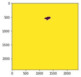
The catchment is only a small proportion of the total dataset, so make sure you apply masking and cropping appropriately.

You will need to develop code to load the time series of snow cover data into a 3D numpy array, cropped to the required catchment

You will then need to develop code to interpolate over any missing data, so that there is an estimate of snow cover for every pixel in the catchment for all days

You will need to produce images (i.e. fully labelled plots) of snow cover spatial data for the catchment for 13 samples spaced equally through the year, one set of images for each year. This will be used to demonstrate that you have achieved this interpolation, so you should show the datyasets for both pre- and post-interpolation.

from geog0111.raster_mask import raster_mask2
import pylab as plt
%matplotlib inline

m = raster_mask2(fname,\
                target_vector_file="data/Hydrological_Units/HUC_Polygons.shp",\
                attribute_filter=2)
plt.imshow(m)

<matplotlib.image.AxesImage at 0x12646fe80>

4.2.3.3 Discharge Data

A sample of the river discharge data are in the file `data/delnorte.dat <data/delnorte.dat>`__.

If you examine the file:

f = open('data/delnorte.dat').readlines()
for i in range(40):
    print(f[i],end='')

# ---------------------------------- WARNING ----------------------------------------
# Provisional data are subject to revision. Go to
# http://help.waterdata.usgs.gov/policies/provisional-data-statement for more information.
#
# File-format description:  http://help.waterdata.usgs.gov/faq/about-tab-delimited-output
# Automated-retrieval info: http://help.waterdata.usgs.gov/faq/automated-retrievals
#
# Contact:   gs-w_support_nwisweb@usgs.gov
# retrieved: 2016-11-02 04:17:13 -04:00     (natwebsdas01)
#
# Data for the following 1 site(s) are contained in this file
#    USGS 08220000 RIO GRANDE NEAR DEL NORTE, CO
# -----------------------------------------------------------------------------------
#
# TS_ID - An internal number representing a time series.
# IV_TS_ID - An internal number representing the Instantaneous Value time series from which the daily statistic is calculated.
#
# Data provided for site 08220000
#    TS_ID       Parameter    Statistic  IV_TS_ID       Description
#    18268       00060        00003      -1             Discharge, cubic feet per second (Mean)
#
# Data-value qualification codes included in this output:
#     A  Approved for publication -- Processing and review completed.
#     e  Value has been edited or estimated by USGS personnel and is write protected.
#
agency_cd   site_no datetime        18268_00060_00003       18268_00060_00003_cd
5s  15s     20d     14n     10s
USGS        08220000        2005-01-01      210     A:e
USGS        08220000        2005-01-02      190     A:e
USGS        08220000        2005-01-03      190     A:e
USGS        08220000        2005-01-04      200     A:e
USGS        08220000        2005-01-05      200     A:e
USGS        08220000        2005-01-06      190     A:e
USGS        08220000        2005-01-07      170     A:e
USGS        08220000        2005-01-08      180     A:e
USGS        08220000        2005-01-09      200     A:e
USGS        08220000        2005-01-10      220     A:e
USGS        08220000        2005-01-11      210     A:e
USGS        08220000        2005-01-12      200     A:e
USGS        08220000        2005-01-13      190     A:e

you will see comment lines that start with #, followed by data lines.

The easiest way to read these data would be to use:

import numpy as np
file = 'data/delnorte.dat'
data = np.loadtxt(file,usecols=(2,3),unpack=True,dtype=str)

# so you have the dates in
# print the first 100
print (data[0][:100])
# and data in
print (data[1][:100])
# but the data start in column 3 so use [2:]

['datetime' '20d' '2005-01-01' '2005-01-02' '2005-01-03' '2005-01-04'
 '2005-01-05' '2005-01-06' '2005-01-07' '2005-01-08' '2005-01-09'
 '2005-01-10' '2005-01-11' '2005-01-12' '2005-01-13' '2005-01-14'
 '2005-01-15' '2005-01-16' '2005-01-17' '2005-01-18' '2005-01-19'
 '2005-01-20' '2005-01-21' '2005-01-22' '2005-01-23' '2005-01-24'
 '2005-01-25' '2005-01-26' '2005-01-27' '2005-01-28' '2005-01-29'
 '2005-01-30' '2005-01-31' '2005-02-01' '2005-02-02' '2005-02-03'
 '2005-02-04' '2005-02-05' '2005-02-06' '2005-02-07' '2005-02-08'
 '2005-02-09' '2005-02-10' '2005-02-11' '2005-02-12' '2005-02-13'
 '2005-02-14' '2005-02-15' '2005-02-16' '2005-02-17' '2005-02-18'
 '2005-02-19' '2005-02-20' '2005-02-21' '2005-02-22' '2005-02-23'
 '2005-02-24' '2005-02-25' '2005-02-26' '2005-02-27' '2005-02-28'
 '2005-03-01' '2005-03-02' '2005-03-03' '2005-03-04' '2005-03-05'
 '2005-03-06' '2005-03-07' '2005-03-08' '2005-03-09' '2005-03-10'
 '2005-03-11' '2005-03-12' '2005-03-13' '2005-03-14' '2005-03-15'
 '2005-03-16' '2005-03-17' '2005-03-18' '2005-03-19' '2005-03-20'
 '2005-03-21' '2005-03-22' '2005-03-23' '2005-03-24' '2005-03-25'
 '2005-03-26' '2005-03-27' '2005-03-28' '2005-03-29' '2005-03-30'
 '2005-03-31' '2005-04-01' '2005-04-02' '2005-04-03' '2005-04-04'
 '2005-04-05' '2005-04-06' '2005-04-07' '2005-04-08']
['18268_00060_00003' '14n' '210' '190' '190' '200' '200' '190' '170' '180'
 '200' '220' '210' '200' '190' '170' '170' '180' '190' '200' '210' '220'
 '220' '220' '220' '220' '220' '220' '230' '240' '230' '210' '200' '190'
 '180' '180' '180' '190' '200' '190' '190' '180' '190' '200' '210' '210'
 '210' '210' '210' '200' '200' '190' '200' '203' '205' '213' '207' '191'
 '190' '196' '190' '195' '196' '194' '189' '201' '201' '208' '218' '233'
 '262' '285' '320' '350' '340' '320' '272' '257' '272' '255' '266' '255'
 '245' '277' '270' '255' '248' '239' '284' '305' '270' '243' '235' '275'
 '344' '401' '424' '430' '576' '705']

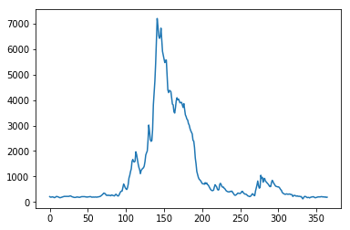
# and the stream flow in data[1][2:]
plt.plot(data[1][2:].astype(float))

[<matplotlib.lines.Line2D at 0x1270929b0>]

You will need to convert the date field (i.e. the data in data[0]) into the day of year.

This is readily accomplished using datetime:

import datetime
# transform the first one, which is data[0][2:]

ds = np.array(data[0][2].split('-')).astype(int)
print (ds)
year,doy = datetime.datetime(ds[0],ds[1],ds[2]).strftime('%Y %j').split()
print (year,doy)

[2005    1    1]
2005 001

4.2.3.4 Temperature data

We can directly access temperature data from here.

The format of `delNorteT.dat <files/data/delNorteT.dat>`__ is given here.

The first three fields are date fields (YEAR, MONTH and DAY), followed by TMAX, TMIN, PRCP, SNOW, SNDP.

You should read in the temperature data for the days and years that you want.

For temperature, you might take a mean of TMAX and TMIN.

Note that these are in Fahrenheit. You should convert them to Celcius.

Note also that there are missing data (values 9998 and 9999). You will need to filter these and interpolate the data in some way. A median might be a good approach, but any interpolation will suffice.

With that processing then, you should have a dataset, Temperature that will look something like (in cyan, for the year 2005):

4.3 Coursework

You need to submit you coursework in the usual manner by the usual submission date.

You must work individually on this task. If you do not, it will be treated as plagiarism. By reading these instructions for this exercise, we assume that you are aware of the UCL rules on plagiarism. You can find more information on this matter in your student handbook. If in doubt about what might constitute plagiarism, ask one of the course convenors.

6.3.1 Summary of coursework requirements

• Part 1: Data Preparation

  The first task you must complete is to produce a dataset of the proportion of HUC catchment 13010001 (Rio Grande headwaters in Colorado, USA) that is covered by snow for two years (not necessarily consecutive), along with associated datasets on temperature (in C) and river discharge at the Del Norte monitoring station. You will use these data in the modelling work in Part 2 of the coursework.

  You may not use data from the years 2005 or 2006, as this will be given to you in illustrations of the material.

  The dataset you produce must have a value for the mean snow cover, temperature and discharge in the catchment for every day over each year.

  Your write up must include fully labelled graph(s) of snow cover, temperature and discharge for the catchment for each year (with units as appropriate), along with some summary statistics (e.g. mean or median, minimum, maximum, and the timing of these).

  You must provide evidence of how you got these data (i.e. the code and commands you ran to produce the data).

Checklist:

* provide fully commented/documented code for all operations.
* provide two years of **daily** data (not 2005 or 2006)
* Generate datasets of:
    * mean snow cover (0.0 to 1.0) for the catchment for each day of the year
    * temperature (C) at the Del Norte monitoring station for each day of the year
    * river discharge at the Del Norte monitoring station for each day of the year
* Produce a table of summary statistics for each of the 3 datasets (one for easch year)
* produce graphs of the 3 datasets for each year (as function of day of year)
* produce an `npz` file containing the 3 datasets, one for each year.
* produce images of snow cover spatial data for the catchment for **13 samples** spaced equally through the year, one set of images for each year. You need to do this for the data pre-interpolation and aftyer you have done the interpolation.

4.3.2 Summary of Advice

The first task involves pulling datasets from different sources. No individual part of that should be too difficult, but you must put this together from the material we have done so far. It is more a question of organisation then.

Perhaps think first about where you want to end up with on this (the ‘output’). This might for example be a dictionary with keys temp, doy, snow and flow, where each of these would be an array with 365 values (or 366 in a leap year).

Then consider the datasets you have: these are: (i) a stack of MODIS data with daily observations; (ii) temperature data in a file; (iii) flow data in a file.

It might be a little fiddly getting the data you want from the flow and temperature data files, but its not very complicated. You will need to consider flagging invalid observations and perhaps interpolating between these.

Processing the MODIS data might take a little more thought, but it is much the same process. Again, we read the datasets in, trying to make this efficient on data size by only using the area of the vector data mask as in a previous exercise. The data reading will be very similar to reading the MODIS LAI product, but you need to work out and implement what changes are necessary. As advised abovem you should use the raster_mask2() function for creating the spatial data masks. Again, you will need to interpolate or perhaps smooth between observations, and then process the snow cover proportions to get an average over the catchment.

The second task revolves around using the model that we have developed above in the function model_accum(). You have been through previous examples in Python where you attempt to estimate some model parameters given an initial estimate of the parameters and some cost function to be minimised. Solving the model calibration part of problem should follow those same lines then. Testing (validation) should be easy enough. Don’t forget to include the estimated parameters (and other relevant information, e.g. your initial estimate, uncertainties if available) in your write up.

There is quite a lot of data presentation here, and you need to provide evidence that you have done the task. Make sure you use images (e.g. of snow cover varying), graphs (e.g. modelled and predicted flow, etc.), and tables (e.g. model parameter estimates) throughout, as appropriate.

If, for some reason, you are unable to complete the first part of the practical, you should submit what you can for that first part, and continue with calibrating the model using the 2005 dataset that we used above. This would be far from ideal as you would not have completed the required elements for either part in that case, but it would generall be better than not submitting anything.

4.3.3 Further advice

There is plenty of scope here for going beyond the basic requirements, if you get time and are interested (and/or want a higher mark!).

You will be given credit for all additional work included in the write up, once you have achieved the basic requirements. So, there is no point (i.e. you will not get credit for) going off on all sorts of interesting lines of exploration here unless you have first completed the core task.

4.3.4 Structure of the Report

The required elements of the report are:

 1. Code for temperature and river discharge data download, reading and saving, with running of code and datasets for 2 years of daily data, and appropriate plots showing the datasets (10%)
     * temperature (C) at the Del Norte monitoring station for each day of the year
     * river discharge at the Del Norte monitoring station for each day of the year

2. Code for downloading MODIS snow cover data, masking, cropping and extracting the data into a 3D numpy array, storing the data, running the code for 2 years data, and appropiate plots. (20%)

3. Code for interpolating MODIS snow cover data and calculating mean snow cover over the catchment, saving the data, running the code for 2 years data, and appropiate plots. (15%)

4. Produce a table of summary statistics for each of the datasets (one for each year) and a `npz` file containing all of the datasets (5%)

For parts 2 and 3, make sure to produce images of snow cover spatial data for the catchment for **13 samples** spaced equally through the year, one set of images for each year. You need to do this for the data pre-interpolation (part 2) and after you have done the interpolation (part 3).

The figures in brackets indicate the percentage of marks that we will award for each section of the report.

4.3.5 Computer Code

General requirements

You will obviously need to submit computer codes as part of this assessment. Some flexibility in the style of these codes is to be expected. For example, some might write a class that encompasses the functionality for all tasks. Some poeple might have multiple versions of codes with different functionality. All of these, and other reasonable variations are allowed.

All codes needed to demonstrate that you have performed the core tasks are required to be included in the submission. You should include all codes that you make use of in the main body of the text in the main body. Any other codes that you want to refer to (e.g. something you tried out as an enhancement and didn’t quite get there) you can include in appendices.

All codes should be well-commented. Part of the marks you get for code will depend on the adequacy of the commenting.

Degree of original work required and plagiarism

If you use a piece of code verbatim that you have taken from the course pages or any other source, you must acknowledge this in comments in your text. Not to do so is plagiarism. Where you have taken some part (e.g. a few lines) of someone else’s code, you should also indicate this. If some of your code is heavily based on code from elsewhere, you must also indicate that.

Some examples.

The first example is guilty of strong plagiarism, it does not seek to acknowledge the source of this code, even though it is just a direct copy, pasted into a method called model():

def model(tempThresh=9.0,K=2000.0,p=0.96):
    '''need to comment this further ...

    '''
    import numpy as np
    meltDays = np.where(temperature > tempThresh)[0]
    accum = snowProportion*0.
    for d in meltDays:
        water = K * snowProportion[d]
        n = np.arange(len(snowProportion)) - d
        m = p ** n
        m[np.where(n<0)]=0
        accum += m * water
    return accum

This is not acceptable.

This should probably be something along the lines of:

def model(tempThresh=9.0,K=2000.0,p=0.96):
    '''need to comment this further ...

    This code is taken directly from
    "Modelling delay in a hydrological network"
    by P. Lewis http://www2.geog.ucl.ac.uk/~plewis/geogg122/DelNorte.html
    and wrapped into a method.
    '''
    # my code: make sure numpy is imported
    import numpy as np

    # code below verbatim from Lewis
    meltDays = np.where(temperature > tempThresh)[0]
    accum = snowProportion*0.
    for d in meltDays:
        water = K * snowProportion[d]
        n = np.arange(len(snowProportion)) - d
        m = p ** n
        m[np.where(n<0)]=0
        accum += m * water
    # my code: return accumulator
    return accum

Now, we acknowledge that this is in essence a direct copy of someone else’s code, and clearly state this. We do also show that we have added some new lines to the code, and that we have wrapped this into a method.

In the next example, we have seen that the way m is generated is in fact rather inefficient, and have re-structured the code. It is partially developed from the original code, and acknowledges this:

def model(tempThresh=9.0,K=2000.0,p=0.96):
    '''need to comment this further ...

    This code after the model developed in
    "Modelling delay in a hydrological network"
    by P. Lewis
    http://www2.geog.ucl.ac.uk/~plewis/geogg122/DelNorte.html

    My modifications have been to make the filtering more efficient.
    '''
    # my code: make sure numpy is imported
    import numpy as np

    # code below verbatim from Lewis unless otherwise indicated
    meltDays = np.where(temperature > tempThresh)[0]
    accum = snowProportion*0.

    # my code: pull the filter block out of the loop
    n = np.arange(len(snowProportion))
    m = p ** n

    for d in meltDays:
        water = K * snowProportion[d]

        # my code: shift the filter on by one day
        # ...do something clever to shift it on by one day

        accum += m * water
    # my code: return accumulator
    return accum

This example makes it clear that significant modifications have been made to the code structure (and probably to its efficiency) although the basic model and looping comes from an existing piece of code. It clearly highlights what the actual modifications have been. Note that this is not a working example!!

Although you are supposed to do this piece of work on your own, there might be some circumstances under which someone has significantly helped you to develop the code (e.g. written the main part of it for you & you’ve just copied that with some minor modifications). You must acknowledge in your code comments if this has happened. On the whole though, this should not occur, as you must complete this work on your own.

If you take a piece of code from somewhere else and all you do is change the variable names and/or other cosmetic changes, you must acknowledge the source of the original code (with a URL if available).

Plagiarism in coding is a tricky issue. One reason for that is that often the best way to learn something like this is to find an example that someone else has written and adapt that to your purposes. Equally, if someone has written some tool/library to do what you want to do, it would generally not be worthwhile for you to write your own but to concentrate on using that to achieve something new. Even in general code writing (i.e. when not submitting it as part of your assessment) you and anyone else who ever has to read your code would find it of value to make reference to where you found the material to base what you did on. The key issue to bear in mind in this work, as it is submitted ‘as your own work’ is that, to avoid being accused of plagiarism and to allow a fair assessment of what you have done, you must clearly acknowledge which parts of it are your own, and the degree to which you could claim them to be your own.

For example, based on … is absolutely fine, and you would certainly be given credit for what you have done. In many circumstances ‘taken verbatim from …’ would also be fine (provided it is acknowledged) but then you would be given credit for what you had done with the code that you had taken from elsewhere (e.g. you find some elegant way of doing the graphs that someone has written and you make use of it for presenting your results).

The difference between what you submit here and the code you might write if this were not a piece submitted for assessment is that you the vast majority of the credit you will gain for the code will be based on the degree to which you demonstrate that you can write code to achieve the required tasks. There would obviously be some credit for taking codes from the coursenotes and bolting them together into something that achieves the overall aim: provided that worked, and you had commented it adequately and acknowledge what the extent of your efforts had been, you should be able to achieve a pass in that component of the work. If there was no original input other than vbolting pieces of existing code together though, you be unlikely to achieve more than a pass. If you get less than a pass in another component of the coursework, that then puts you in danger of an overall fail.

Provided you achieve the core tasks, the more original work that you do/show (that is of good quality), the higher the mark you will get. Once you have achieved the core tasks, even if you try something and don’t quite achieve it, is is probably worth including, as you may get marks for what you have done (or that fact that it was a good or interesting thing to try to do).

Documentation

Note: All methods/functions and classes must be documented for the code to be adequate. Generally, this will contain:

• some text on the purpose of the method (/function/class)
• some text describing the inputs and outputs, including reference to any relevant details such as datatype, shape etc where such things are of relevance to understanding the code.
• some text on keywords, e.g.:

def complex(real=0.0, imag=0.0):
    """Form a complex number.

    Keyword arguments:
    real -- the real part (default 0.0)
    imag -- the imaginary part (default 0.0)

    Example taken verbatim from:
    http://www.python.org/dev/peps/pep-0257/
    """
    if imag == 0.0 and real == 0.0: return complex_zero

You should look at the document on good docstring conventions when considering how to document methods, classes etc.

To demonstrate your documentation, you must include the help text generated by your code after you include the code. e.g.:

def print_something(this,stderr=False):
    '''This does something.

    Keyword arguments:
    stderr -- set to True to print to stderr (default False)
    '''

    if stderr:
        # import sys.stderr
        from sys import stderr

        # print to stderr channel, converting this to str
        print >> stderr,str(this)

        # job done, return
        return

    # print to stdout, converting this to str
    print (str(this))

    return

Then the help text would be:

help(print_something)

Help on function print_something in module __main__:

print_something(this, stderr=False)
    This does something.

    Keyword arguments:
    stderr -- set to True to print to stderr (default False)

The above example represents a ‘good’ level of commenting as the code broadly adheres to the style suggestions and most of the major features are covered. It is not quite ‘very good/excellent’ as the description of the purpose of the method (rather important) is trivial and it fails to describe the input this in any way. An excellent piece would do all of these things, and might well tell us about any dependencies (e.g. requires sys if stderr set to True).

An inadequate example would be:

def print_something(this,stderr=False):
    '''This prints something'''
    if stderr:
        from sys import stderr
        print >> stderr,str(this)
        return
    print (str(this))

It is inadequate because it still only has a trivial description of the purpose of the method, it tells us nothing about inputs/outputs and there is no commenting inside the method.

Word limit

There is no word limit per se on the computer codes, though as with all writing, you should try to be succint rather than overly verbose.

Code style

A good to excellent piece of code would take into account issues raised in the style guide. The ‘degree of excellence’ would depend on how well you take those points on board.