Table of Contents
3.4 Stacking and interpolating data
3.4.1 Introduction
3.4.1.1 Test your login
3.4.2 QA data
3.4.2.1 Why QA data?
3.4.2.2 Set condition variables
3.4.2.3 interpreting QA
3.4.2.4 Deriving a weight from QA
3.4.3 A time series
3.4.4 Weighted interpolation
3.4.4.1 Smoothing
3.4.5 Making movies
3.4.5.1 Javascript HTML
3.4.5.2 Animated gif
3.4 Stacking and interpolating data
3.4.1 Introduction
In this section, we will:
- develop code to produce a stacked dataset of spatio-temporal data on a grid
- interpolate over any missing data
- smooth the dataset
3.4.1.1 Test your login
Let’s first test your NASA login:
z = 37373676
try:
print(z)
except (NameError):
print("Variable z is not defined")
37373676
import geog0111.nasa_requests as nasa_requests
from geog0111.cylog import cylog
url = 'https://e4ftl01.cr.usgs.gov/MOTA/MCD15A3H.006/2018.09.30/'
# grab the HTML information
try:
html = nasa_requests.get(url).text
# test a few lines of the html
if html[:20] == '<!DOCTYPE HTML PUBLI':
print('this seems to be ok ... ')
print(
'use cylog().login() anywhere you need to specify the tuple (username,password)'
)
except:
print('login error ... ')
print('try entering your username password again')
print('then re-run this cell until it works')
print('If its wednesday, ignore this!')
# uncomment next line to reset password
#cylog(init=True)
this seems to be ok ...
use cylog().login() anywhere you need to specify the tuple (username,password)
# get the MODIS LAI dataset for 2016/2017 for W. Europe
from geog0111.geog_data import procure_dataset
from pathlib import Path
files = list(Path('data').glob('MCD15A3H.A201[6-7]*h1[7-8]v0[3-4].006*hdf'))
if len(files) < 732:
_ = procure_dataset("lai_files",verbose=False)
import gdal
import matplotlib.pyplot as plt
%matplotlib inline
g = gdal.Open("data/MCD15A3H.A2016001.h18v03.006.2016007073724.hdf")
sds = g.GetSubDatasets()
for s in sds:
print(s[1])
[2400x2400] Fpar_500m MOD_Grid_MCD15A3H (8-bit unsigned integer)
[2400x2400] Lai_500m MOD_Grid_MCD15A3H (8-bit unsigned integer)
[2400x2400] FparLai_QC MOD_Grid_MCD15A3H (8-bit unsigned integer)
[2400x2400] FparExtra_QC MOD_Grid_MCD15A3H (8-bit unsigned integer)
[2400x2400] FparStdDev_500m MOD_Grid_MCD15A3H (8-bit unsigned integer)
[2400x2400] LaiStdDev_500m MOD_Grid_MCD15A3H (8-bit unsigned integer)
Now make sure you have the world borders ESRI shape file you need:
import requests
import shutil
from pathlib import Path
# zip file
zipfile = 'TM_WORLD_BORDERS-0.3.zip'
# URL
tm_borders_url = f"http://thematicmapping.org/downloads/{zipfile}"
# destibnation folder
destination_folder = Path('data')
# set up some filenames
zip_file = destination_folder.joinpath(zipfile)
shape_file = zip_file.with_name(zipfile.replace('zip', 'shp'))
# download zip if need to
if not Path(zip_file).exists():
r = requests.get(tm_borders_url)
with open(zip_file, 'wb') as fp:
fp.write(r.content)
# extract shp from zip if need to
if not Path(shape_file).exists():
shutil.unpack_archive(zip_file.as_posix(), extract_dir=destination_folder)
3.4.2 QA data
3.4.2.1 Why QA data?
The quality of data varies according to sampling and other factors. For satellite-derived data using optical wavelengths, the two main controls are orbital constraints and cloud cover. We generally define a ‘quaity’ data layer to express this.
To use a satellite-derived dataset, we need to look at ‘quality’ data for dataset (and/or uncertainty).
For example, if interpolating data, we would want to base the weight we put on any sample on the ‘quality’ of that sample. This will be expressed by either some QC (Quality Control) assessment (‘good’, ‘ok’, ‘bad’) or some measure of uncertainty (or both).
Here, we will use the QA information in the LAI product to generate a sample weighting scheme. We shall later use this weighting for data smoothing and interpolation.
First, let’s access the LAI and QA datasets.
We can do this by specifying either Lai_500m or FparLai_QC in
the dataset label.
3.4.2.2 Set condition variables
Let’s set up the variables we will use, including a pattern to match the
tile information we need.
Here, we have:
tile = 'h1[7-8]v0[3-4]'
which we can interpret as:
h17v03, h17v04, h18v03, or h18v04
The tile definition ius useful for us to use in any output names (so we
can identify it from the name). But the string h1[7-8]v0[3-4]
contains some ‘awkward’ characters, namely [, ] and - that
we might prefer not to use in a filename.
So we derive a new descriptor that we call tile_ which is more
‘filename friendly’.
Thye rest of the code below proceeds much the same as code we have previously used.
We build a gdal VRT file from the set of hdf files using
gdal.BuildVRT().
Then we crop to the vector defined by the FIPS variable in the
shapefile (the country code here) using gdal.Warp(). We save this as
a gdal VRT file, decsribed by the variable clipped_file.
When we make gdal calls, we need to force the system to write files to
disc. This can be done by closing the (effective) file descriptors, or
by deleting the variable g in this case. If you don’t do that, you
can hit file synchronisation problems. You should always close (or
delete) file descriptors when you have finished with them.
You should be able to follow what goes on in the code block below. We will re-use these same ideas later, so it is worthwhile understanding the steps we go through now.
import gdal
import numpy as np
from pathlib import Path
from geog0111.create_blank_file import create_blank_file
from datetime import datetime
#-----------------
# set up the dataset information
destination_folder = Path('data')
year = 2017
product = 'MCD15A3H'
version = 6
tile = 'h1[7-8]v0[3-4]'
doy = 149
params = ['Lai_500m', 'FparLai_QC']
# Luxembourg
FIPS = "LU"
#-----------------
# make a text-friendly version of tile
tile_ = tile.replace('[','_').replace(']','_').replace('-','')+FIPS
# location of the shapefile
shape_file = destination_folder.\
joinpath('TM_WORLD_BORDERS-0.3.shp').as_posix()
# define strings for the ip and op files
ipfile = destination_folder.\
joinpath(f'{product}.A{year}{doy:03d}.{tile_}.{version:03d}').as_posix()
opfile = ipfile.replace(f'{doy:03d}.','').replace(tile,tile_)
print('ipfile',ipfile)
print('opfile',opfile)
# now glob the hdf files matching the pattern
filenames = list(destination_folder\
.glob(f'{product}.A{year}{doy:03d}.{tile}.{version:03d}.*.hdf'))
# start with an empty list
ofiles = []
# loop over each parameter we need
for d in params:
gdal_filenames = []
for file_name in filenames:
fname = f'HDF4_EOS:EOS_GRID:'+\
f'"{file_name.as_posix()}":'+\
f'MOD_Grid_MCD15A3H:{d}'
gdal_filenames.append(fname)
dataset_names = sorted(gdal_filenames)
# mangle the dataset names
dataset_names = sorted([f'HDF4_EOS:EOS_GRID:'+\
f'"{file_name.as_posix()}":'+\
f'MOD_Grid_MCD15A3H:{d}'\
for file_name in filenames])
print(dataset_names)
# derive some filenames for vrt files
spatial_file = f'{opfile}.{doy:03d}.{d}.vrt'
clipped_file = f'{opfile}.{doy:03d}_clip.{d}.vrt'
# build the files
g = gdal.BuildVRT(spatial_file, dataset_names)
if(g):
del(g)
g = gdal.Warp(clipped_file,\
spatial_file,\
format='VRT', dstNodata=255,\
cutlineDSName=shape_file,\
cutlineWhere=f"FIPS='{FIPS}'",\
cropToCutline=True)
if (g):
del(g)
ofiles.append(clipped_file)
print(ofiles)
ipfile data/MCD15A3H.A2017149.h1_78_v0_34_LU.006
opfile data/MCD15A3H.A2017h1_78_v0_34_LU.006
['HDF4_EOS:EOS_GRID:"data/MCD15A3H.A2017149.h17v03.006.2017164112436.hdf":MOD_Grid_MCD15A3H:Lai_500m', 'HDF4_EOS:EOS_GRID:"data/MCD15A3H.A2017149.h17v04.006.2017164112432.hdf":MOD_Grid_MCD15A3H:Lai_500m', 'HDF4_EOS:EOS_GRID:"data/MCD15A3H.A2017149.h18v03.006.2017164112435.hdf":MOD_Grid_MCD15A3H:Lai_500m', 'HDF4_EOS:EOS_GRID:"data/MCD15A3H.A2017149.h18v04.006.2017164112441.hdf":MOD_Grid_MCD15A3H:Lai_500m']
['HDF4_EOS:EOS_GRID:"data/MCD15A3H.A2017149.h17v03.006.2017164112436.hdf":MOD_Grid_MCD15A3H:FparLai_QC', 'HDF4_EOS:EOS_GRID:"data/MCD15A3H.A2017149.h17v04.006.2017164112432.hdf":MOD_Grid_MCD15A3H:FparLai_QC', 'HDF4_EOS:EOS_GRID:"data/MCD15A3H.A2017149.h18v03.006.2017164112435.hdf":MOD_Grid_MCD15A3H:FparLai_QC', 'HDF4_EOS:EOS_GRID:"data/MCD15A3H.A2017149.h18v04.006.2017164112441.hdf":MOD_Grid_MCD15A3H:FparLai_QC']
['data/MCD15A3H.A2017h1_78_v0_34_LU.006.149_clip.Lai_500m.vrt', 'data/MCD15A3H.A2017h1_78_v0_34_LU.006.149_clip.FparLai_QC.vrt']
import gdal
import numpy as np
from pathlib import Path
from geog0111.create_blank_file import create_blank_file
from datetime import datetime, timedelta
def find_mcdfiles(year, doy, tiles, folder):
data_folder = Path(folder)
# Find all MCD files
mcd_files = []
for tile in tiles:
sel_files = data_folder.glob(
f"MCD15*.A{year:d}{doy:03d}.{tile:s}.*hdf")
for fich in sel_files:
mcd_files.append(fich)
return mcd_files
def create_gdal_friendly_names(filenames, layer):
# Create GDAL friendly-names...
gdal_filenames = []
for file_name in filenames:
fname = f'HDF4_EOS:EOS_GRID:'+\
f'"{file_name.as_posix()}":'+\
f'MOD_Grid_MCD15A3H:{layer:s}'
gdal_filenames.append(fname)
return gdal_filenames
def mosaic_and_clip(tiles,
doy,
year,
folder="data/",
layer="Lai_500m",
shpfile="data/TM_WORLD_BORDERS-0.3.shp",
country_code="LU"):
folder_path = Path(folder)
# Find all files to mosaic together
hdf_files = find_mcdfiles(year, doy, tiles, folder)
# Create GDAL friendly-names...
gdal_filenames = create_gdal_friendly_names(hdf_files, layer)
g = gdal.Warp(
"",
gdal_filenames,
format="MEM",
dstNodata=255,
cutlineDSName=shpfile,
cutlineWhere=f"FIPS='{country_code:s}'",
cropToCutline=True)
data = g.ReadAsArray()
return data
output = np.zeros((176, 123, 85))
today = datetime(2017, 1, 1)
for time in range(85):
if today.year != 2017:
break
doy = int(today.strftime("%j"))
print(today, doy)
LU_mosaic = mosaic_and_clip(["h17v03", "h17v04", "h18v03", "h18v04"], doy, 2017)
output[:, :, time] = LU_mosaic
today = today + timedelta(days=4)
2017-01-01 00:00:00 1
2017-01-05 00:00:00 5
2017-01-09 00:00:00 9
2017-01-13 00:00:00 13
2017-01-17 00:00:00 17
2017-01-21 00:00:00 21
2017-01-25 00:00:00 25
2017-01-29 00:00:00 29
2017-02-02 00:00:00 33
2017-02-06 00:00:00 37
2017-02-10 00:00:00 41
2017-02-14 00:00:00 45
2017-02-18 00:00:00 49
2017-02-22 00:00:00 53
2017-02-26 00:00:00 57
2017-03-02 00:00:00 61
2017-03-06 00:00:00 65
2017-03-10 00:00:00 69
2017-03-14 00:00:00 73
2017-03-18 00:00:00 77
2017-03-22 00:00:00 81
2017-03-26 00:00:00 85
2017-03-30 00:00:00 89
2017-04-03 00:00:00 93
2017-04-07 00:00:00 97
2017-04-11 00:00:00 101
2017-04-15 00:00:00 105
2017-04-19 00:00:00 109
2017-04-23 00:00:00 113
2017-04-27 00:00:00 117
2017-05-01 00:00:00 121
2017-05-05 00:00:00 125
2017-05-09 00:00:00 129
2017-05-13 00:00:00 133
2017-05-17 00:00:00 137
2017-05-21 00:00:00 141
2017-05-25 00:00:00 145
2017-05-29 00:00:00 149
2017-06-02 00:00:00 153
2017-06-06 00:00:00 157
2017-06-10 00:00:00 161
2017-06-14 00:00:00 165
2017-06-18 00:00:00 169
2017-06-22 00:00:00 173
2017-06-26 00:00:00 177
2017-06-30 00:00:00 181
2017-07-04 00:00:00 185
2017-07-08 00:00:00 189
2017-07-12 00:00:00 193
2017-07-16 00:00:00 197
2017-07-20 00:00:00 201
2017-07-24 00:00:00 205
2017-07-28 00:00:00 209
2017-08-01 00:00:00 213
2017-08-05 00:00:00 217
2017-08-09 00:00:00 221
2017-08-13 00:00:00 225
2017-08-17 00:00:00 229
2017-08-21 00:00:00 233
2017-08-25 00:00:00 237
2017-08-29 00:00:00 241
2017-09-02 00:00:00 245
2017-09-06 00:00:00 249
2017-09-10 00:00:00 253
2017-09-14 00:00:00 257
2017-09-18 00:00:00 261
2017-09-22 00:00:00 265
2017-09-26 00:00:00 269
2017-09-30 00:00:00 273
2017-10-04 00:00:00 277
2017-10-08 00:00:00 281
2017-10-12 00:00:00 285
2017-10-16 00:00:00 289
2017-10-20 00:00:00 293
2017-10-24 00:00:00 297
2017-10-28 00:00:00 301
2017-11-01 00:00:00 305
2017-11-05 00:00:00 309
2017-11-09 00:00:00 313
2017-11-13 00:00:00 317
2017-11-17 00:00:00 321
2017-11-21 00:00:00 325
2017-11-25 00:00:00 329
2017-11-29 00:00:00 333
2017-12-03 00:00:00 337
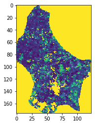
plt.imshow(output[:, :, 50], vmin=0, vmax=80)
<matplotlib.image.AxesImage at 0x120defda0>
Exercise 3.4.1
- examine the code block above, and write a function that takes as
inputs the variables given in the block enclosed by
#-----------------, the dataset information - the code should setup the VRT files and return the list of clipped
dataset filenames:
['data/MCD15A3H.A2017h1_78_v0_34_LU.006.149_clip.Lai_500m.vrt', 'data/MCD15A3H.A2017h1_78_v0_34_LU.006.149_clip.FparLai_QC.vrt']here. - Make sure you test your function: check that it generates the files you expect from the inputs you give.
- try to develop an automated test to see that it has worked (Homework)
Hint
Be clear about what you are doing in your code.
The purpose of this function is to build clipped VRT files for the conditions you set.
The conditions are the parameters driving the function.
The list of files you develop are returned.
# do exercise here
An attempt at some of this is to try to split the code given cell into a few self-contained and easily testable functions. Broadly speaking, what the code does is
- Create a list of HDF files that match a pattern (date stamp, as well as belonging to a set of tiles)
- For each HDF file, select a layer using the GDAL selection method
- Mosaic all the files for the given date
- Apply a clipping mask from a vector file
Points 3 and 4 are really direct calls to GDAL functions, and can be combined into one, but we can spin off two simple functions for the first two tasks.
Finding the files requires knowledge of the dates (day of year and
year), the location of the files (a folder), as well as the tiles.
Rather than use a complex wildcard/regular expression like
h1[7-8]v0[3-4], we can just pass a list of tiles and loop over them.
We return the filenames. In the available dataset, we have a couple of
years of data with four tiles, so we can test this by checking that we
get four tiles for different dates.
def find_mcdfiles(year, doy, tiles, folder):
"""Finds MCD15 files in a given folder for a date and set of tiles
#TODO Missing documentation
"""
data_folder = Path(folder)
# Find all MCD files
mcd_files = []
for tile in tiles:
# Loop over all tiles, and search for files that have
# the tile of interest
sel_files = data_folder.glob(
f"MCD15*.A{year:d}{doy:03d}.{tile:s}.*hdf")
for fich in sel_files:
mcd_files.append(fich)
return mcd_files
# Test with two dates
results = find_mcdfiles(2017, 1, ["h17v03", "h17v04", "h18v03", "h18v04"],
folder="data/")
for result in results:
print(result)
results = find_mcdfiles(2017, 45, ["h17v03", "h17v04", "h18v03", "h18v04"],
folder="data/")
for result in results:
print(result)
data/MCD15A3H.A2017001.h17v03.006.2017014005341.hdf
data/MCD15A3H.A2017001.h17v04.006.2017014005344.hdf
data/MCD15A3H.A2017001.h18v03.006.2017014005401.hdf
data/MCD15A3H.A2017001.h18v04.006.2017014005359.hdf
data/MCD15A3H.A2017045.h17v03.006.2017053101326.hdf
data/MCD15A3H.A2017045.h17v04.006.2017053101338.hdf
data/MCD15A3H.A2017045.h18v03.006.2017053101154.hdf
data/MCD15A3H.A2017045.h18v04.006.2017053101351.hdf
The second bit of code broadly speaking just embellishes the previous file names by giving them a path to the internal dataset that GDAL can read. For the MCD15A3H product, this means that we build a string with the filename and the layer as
HDF4_EOS:EOS_GRID:"<the filename>":MOD_Grid_MCD15A3H:<the layer>
Already, we can see that f-strings will be a very good fit for this! As
a testing framework for this function, we ought to be able to open the
files with gdal.Open and get some numbers…
def create_gdal_friendly_names(filenames, layer):
"""Given a list of HDF filenames, and a layer, create
a list of GDAL pointers to an internal layer in the
filenames given.
#TODO docstring needs improvements
"""
# Create GDAL friendly-names...
gdal_filenames = []
for file_name in filenames:
# Convert filename to a string. Could also do it with
# str(file_name)
fname = file_name.as_posix()
# Create the GDAL pointer name
fname = f'HDF4_EOS:EOS_GRID:"{fname:s}":MOD_Grid_MCD15A3H:{layer:s}'
gdal_filenames.append(fname)
return gdal_filenames
# Testing! Get some filenames from find_mcdfiles....
results = find_mcdfiles(2017, 45, ["h17v03", "h17v04", "h18v03", "h18v04"],
folder="data/")
gdal_filenames = create_gdal_friendly_names(results, "Lai_500m")
for gname in gdal_filenames:
print(gdal.Info(gname, stats=True))
break
# Check another layer...
gdal_filenames = create_gdal_friendly_names(results, "FparLai_QC")
for gname in gdal_filenames:
print(gdal.Info(gname, stats=True))
break
Driver: HDF4Image/HDF4 Dataset
Files: data/MCD15A3H.A2017045.h17v03.006.2017053101326.hdf
Size is 2400, 2400
Coordinate System is:
PROJCS["unnamed",
GEOGCS["Unknown datum based upon the custom spheroid",
DATUM["Not specified (based on custom spheroid)",
SPHEROID["Custom spheroid",6371007.181,0]],
PRIMEM["Greenwich",0],
UNIT["degree",0.0174532925199433]],
PROJECTION["Sinusoidal"],
PARAMETER["longitude_of_center",0],
PARAMETER["false_easting",0],
PARAMETER["false_northing",0],
UNIT["Meter",1]]
Origin = (-1111950.519667000044137,6671703.117999999783933)
Pixel Size = (463.312716527916677,-463.312716527916507)
Metadata:
add_offset=0
add_offset_err=0
ALGORITHMPACKAGEACCEPTANCEDATE=10-01-2004
ALGORITHMPACKAGEMATURITYCODE=Normal
ALGORITHMPACKAGENAME=MCDPR_15A3
ALGORITHMPACKAGEVERSION=6
ASSOCIATEDINSTRUMENTSHORTNAME.1=MODIS
ASSOCIATEDINSTRUMENTSHORTNAME.2=MODIS
ASSOCIATEDPLATFORMSHORTNAME.1=Terra
ASSOCIATEDPLATFORMSHORTNAME.2=Aqua
ASSOCIATEDSENSORSHORTNAME.1=MODIS
ASSOCIATEDSENSORSHORTNAME.2=MODIS
AUTOMATICQUALITYFLAG.1=Passed
AUTOMATICQUALITYFLAGEXPLANATION.1=No automatic quality assessment is performed in the PGE
calibrated_nt=21
CHARACTERISTICBINANGULARSIZE500M=15.0
CHARACTERISTICBINSIZE500M=463.312716527778
DATACOLUMNS500M=2400
DATAROWS500M=2400
DAYNIGHTFLAG=Day
DESCRREVISION=6.0
EASTBOUNDINGCOORDINATE=0.016666666662491
ENGINEERING_DATA=(none-available)
EXCLUSIONGRINGFLAG.1=N
GEOANYABNORMAL=False
GEOESTMAXRMSERROR=50.0
GLOBALGRIDCOLUMNS500M=86400
GLOBALGRIDROWS500M=43200
GRANULEBEGINNINGDATETIME=2017-02-16T10:25:37.000Z
GRANULEDAYNIGHTFLAG=Day
GRANULEENDINGDATETIME=2017-02-16T10:25:37.000Z
GRINGPOINTLATITUDE.1=49.7394264948349, 59.9999999946118, 60.0089388384779, 49.7424953501575
GRINGPOINTLONGITUDE.1=-15.4860189105775, -19.9999999949462, 0.0325645816155362, 0.0125638874822839
GRINGPOINTSEQUENCENO.1=1, 2, 3, 4
HDFEOSVersion=HDFEOS_V2.17
HORIZONTALTILENUMBER=17
identifier_product_doi=10.5067/MODIS/MCD15A3H.006
identifier_product_doi=10.5067/MODIS/MCD15A3H.006
identifier_product_doi_authority=http://dx.doi.org
identifier_product_doi_authority=http://dx.doi.org
INPUTPOINTER=MYD15A1H.A2017048.h17v03.006.2017050060914.hdf, MYD15A1H.A2017047.h17v03.006.2017049094106.hdf, MYD15A1H.A2017046.h17v03.006.2017048064901.hdf, MYD15A1H.A2017045.h17v03.006.2017047060809.hdf, MOD15A1H.A2017048.h17v03.006.2017050103059.hdf, MOD15A1H.A2017047.h17v03.006.2017053100630.hdf, MOD15A1H.A2017046.h17v03.006.2017052201108.hdf, MOD15A1H.A2017045.h17v03.006.2017047102537.hdf, MCD15A3_ANC_RI4.hdf
LOCALGRANULEID=MCD15A3H.A2017045.h17v03.006.2017053101326.hdf
LOCALVERSIONID=5.0.4
LONGNAME=MODIS/Terra+Aqua Leaf Area Index/FPAR 4-Day L4 Global 500m SIN Grid
long_name=MCD15A3H MODIS/Terra Gridded 500M Leaf Area Index LAI (4-day composite)
MAXIMUMOBSERVATIONS500M=1
MOD15A1_ANC_BUILD_CERT=mtAncUtil v. 1.8 Rel. 09.11.2000 17:36 API v. 2.5.6 release 09.14.2000 16:33 Rev.Index 102 (J.Glassy)
MOD15A2_FILLVALUE_DOC=MOD15A2 FILL VALUE LEGEND
255 = _Fillvalue, assigned when:
* the MOD09GA suf. reflectance for channel VIS, NIR was assigned its _Fillvalue, or
* land cover pixel itself was assigned _Fillvalus 255 or 254.
254 = land cover assigned as perennial salt or inland fresh water.
253 = land cover assigned as barren, sparse vegetation (rock, tundra, desert.)
252 = land cover assigned as perennial snow, ice.
251 = land cover assigned as "permanent" wetlands/inundated marshlands.
250 = land cover assigned as urban/built-up.
249 = land cover assigned as "unclassified" or not able to determine.
MOD15A2_FparExtra_QC_DOC=
FparExtra_QC 6 BITFIELDS IN 8 BITWORD
LANDSEA PASS-THROUGH START 0 END 1 VALIDS 4
LANDSEA 00 = 0 LAND AggrQC(3,5)values{001}
LANDSEA 01 = 1 SHORE AggrQC(3,5)values{000,010,100}
LANDSEA 10 = 2 FRESHWATER AggrQC(3,5)values{011,101}
LANDSEA 11 = 3 OCEAN AggrQC(3,5)values{110,111}
SNOW_ICE (from Aggregate_QC bits) START 2 END 2 VALIDS 2
SNOW_ICE 0 = No snow/ice detected
SNOW_ICE 1 = Snow/ice were detected
AEROSOL START 3 END 3 VALIDS 2
AEROSOL 0 = No or low atmospheric aerosol levels detected
AEROSOL 1 = Average or high aerosol levels detected
CIRRUS (from Aggregate_QC bits {8,9} ) START 4 END 4 VALIDS 2
CIRRUS 0 = No cirrus detected
CIRRUS 1 = Cirrus was detected
INTERNAL_CLOUD_MASK START 5 END 5 VALIDS 2
INTERNAL_CLOUD_MASK 0 = No clouds
INTERNAL_CLOUD_MASK 1 = Clouds were detected
CLOUD_SHADOW START 6 END 6 VALIDS 2
CLOUD_SHADOW 0 = No cloud shadow detected
CLOUD_SHADOW 1 = Cloud shadow detected
SCF_BIOME_MASK START 7 END 7 VALIDS 2
SCF_BIOME_MASK 0 = Biome outside interval <1,4>
SCF_BIOME_MASK 1 = Biome in interval <1,4>
MOD15A2_FparLai_QC_DOC=
FparLai_QC 5 BITFIELDS IN 8 BITWORD
MODLAND_QC START 0 END 0 VALIDS 2
MODLAND_QC 0 = Good Quality (main algorithm with or without saturation)
MODLAND_QC 1 = Other Quality (back-up algorithm or fill value)
SENSOR START 1 END 1 VALIDS 2
SENSOR 0 = Terra
SENSOR 1 = Aqua
DEADDETECTOR START 2 END 2 VALIDS 2
DEADDETECTOR 0 = Detectors apparently fine for up to 50% of channels 1,2
DEADDETECTOR 1 = Dead detectors caused >50% adjacent detector retrieval
CLOUDSTATE START 3 END 4 VALIDS 4 (this inherited from Aggregate_QC bits {0,1} cloud state)
CLOUDSTATE 00 = 0 Significant clouds NOT present (clear)
CLOUDSTATE 01 = 1 Significant clouds WERE present
CLOUDSTATE 10 = 2 Mixed cloud present on pixel
CLOUDSTATE 11 = 3 Cloud state not defined,assumed clear
SCF_QC START 5 END 7 VALIDS 5
SCF_QC 000=0 Main (RT) algorithm used, best result possible (no saturation)
SCF_QC 001=1 Main (RT) algorithm used, saturation occured. Good, very usable.
SCF_QC 010=2 Main algorithm failed due to bad geometry, empirical algorithm used
SCF_QC 011=3 Main algorithm faild due to problems other than geometry, empirical algorithm used
SCF_QC 100=4 Pixel not produced at all, value coudn't be retrieved (possible reasons: bad L1B data, unusable MOD09GA data)
MOD15A2_StdDev_QC_DOC=MOD15A2 STANDARD DEVIATION FILL VALUE LEGEND
255 = _Fillvalue, assigned when:
* the MOD09GA suf. reflectance for channel VIS, NIR was assigned its _Fillvalue, or
* land cover pixel itself was assigned _Fillvalus 255 or 254.
254 = land cover assigned as perennial salt or inland fresh water.
253 = land cover assigned as barren, sparse vegetation (rock, tundra, desert.)
252 = land cover assigned as perennial snow, ice.
251 = land cover assigned as "permanent" wetlands/inundated marshlands.
250 = land cover assigned as urban/built-up.
249 = land cover assigned as "unclassified" or not able to determine.
248 = no standard deviation available, pixel produced using backup method.
NADIRDATARESOLUTION500M=500m
NDAYS_COMPOSITED=8
NORTHBOUNDINGCOORDINATE=59.9999999946118
NUMBEROFGRANULES=1
PARAMETERNAME.1=MCDPR15A3H
PGEVERSION=6.0.5
PROCESSINGCENTER=MODAPS
PROCESSINGENVIRONMENT=Linux minion6010 2.6.32-642.6.2.el6.x86_64 #1 SMP Wed Oct 26 06:52:09 UTC 2016 x86_64 x86_64 x86_64 GNU/Linux
PRODUCTIONDATETIME=2017-02-22T10:13:27.000Z
QAPERCENTCLOUDCOVER.1=12
QAPERCENTEMPIRICALMODEL=30
QAPERCENTGOODFPAR=70
QAPERCENTGOODLAI=70
QAPERCENTGOODQUALITY=70
QAPERCENTINTERPOLATEDDATA.1=0
QAPERCENTMAINMETHOD=70
QAPERCENTMISSINGDATA.1=77
QAPERCENTOTHERQUALITY=100
QAPERCENTOUTOFBOUNDSDATA.1=77
RANGEBEGINNINGDATE=2017-02-14
RANGEBEGINNINGTIME=00:00:00
RANGEENDINGDATE=2017-02-17
RANGEENDINGTIME=23:59:59
REPROCESSINGACTUAL=reprocessed
REPROCESSINGPLANNED=further update is anticipated
scale_factor=0.1
scale_factor_err=0
SCIENCEQUALITYFLAG.1=Not Investigated
SCIENCEQUALITYFLAGEXPLANATION.1=See http://landweb.nascom/nasa.gov/cgi-bin/QA_WWW/qaFlagPage.cgi?sat=aqua the product Science Quality status.
SHORTNAME=MCD15A3H
SOUTHBOUNDINGCOORDINATE=49.9999999955098
SPSOPARAMETERS=5367, 2680
SYSTEMFILENAME=MYD15A1H.A2017048.h17v03.006.2017050060914.hdf, MYD15A1H.A2017047.h17v03.006.2017049094106.hdf, MYD15A1H.A2017046.h17v03.006.2017048064901.hdf, MYD15A1H.A2017045.h17v03.006.2017047060809.hdf, MOD15A1H.A2017048.h17v03.006.2017050103059.hdf, MOD15A1H.A2017047.h17v03.006.2017053100630.hdf, MOD15A1H.A2017046.h17v03.006.2017052201108.hdf, MOD15A1H.A2017045.h17v03.006.2017047102537.hdf
TileID=51017003
UM_VERSION=U.MONTANA MODIS PGE34 Vers 5.0.4 Rev 4 Release 10.18.2006 23:59
units=m^2/m^2
valid_range=0, 100
VERSIONID=6
VERTICALTILENUMBER=03
WESTBOUNDINGCOORDINATE=-19.9999999949462
_FillValue=255
Corner Coordinates:
Upper Left (-1111950.520, 6671703.118) ( 20d 0' 0.00"W, 60d 0' 0.00"N)
Lower Left (-1111950.520, 5559752.598) ( 15d33'26.06"W, 50d 0' 0.00"N)
Upper Right ( 0.000, 6671703.118) ( 0d 0' 0.01"E, 60d 0' 0.00"N)
Lower Right ( 0.000, 5559752.598) ( 0d 0' 0.01"E, 50d 0' 0.00"N)
Center ( -555975.260, 6115727.858) ( 8d43' 2.04"W, 55d 0' 0.00"N)
Band 1 Block=2400x416 Type=Byte, ColorInterp=Gray
Description = MCD15A3H MODIS/Terra Gridded 500M Leaf Area Index LAI (4-day composite)
Minimum=0.000, Maximum=254.000, Mean=197.581, StdDev=103.876
NoData Value=255
Unit Type: m^2/m^2
Offset: 0, Scale:0.1
Metadata:
STATISTICS_MAXIMUM=254
STATISTICS_MEAN=197.5806692449
STATISTICS_MINIMUM=0
STATISTICS_STDDEV=103.87553463306
Driver: HDF4Image/HDF4 Dataset
Files: data/MCD15A3H.A2017045.h17v03.006.2017053101326.hdf
data/MCD15A3H.A2017045.h17v03.006.2017053101326.hdf.aux.xml
Size is 2400, 2400
Coordinate System is:
PROJCS["unnamed",
GEOGCS["Unknown datum based upon the custom spheroid",
DATUM["Not specified (based on custom spheroid)",
SPHEROID["Custom spheroid",6371007.181,0]],
PRIMEM["Greenwich",0],
UNIT["degree",0.0174532925199433]],
PROJECTION["Sinusoidal"],
PARAMETER["longitude_of_center",0],
PARAMETER["false_easting",0],
PARAMETER["false_northing",0],
UNIT["Meter",1]]
Origin = (-1111950.519667000044137,6671703.117999999783933)
Pixel Size = (463.312716527916677,-463.312716527916507)
Metadata:
ALGORITHMPACKAGEACCEPTANCEDATE=10-01-2004
ALGORITHMPACKAGEMATURITYCODE=Normal
ALGORITHMPACKAGENAME=MCDPR_15A3
ALGORITHMPACKAGEVERSION=6
ASSOCIATEDINSTRUMENTSHORTNAME.1=MODIS
ASSOCIATEDINSTRUMENTSHORTNAME.2=MODIS
ASSOCIATEDPLATFORMSHORTNAME.1=Terra
ASSOCIATEDPLATFORMSHORTNAME.2=Aqua
ASSOCIATEDSENSORSHORTNAME.1=MODIS
ASSOCIATEDSENSORSHORTNAME.2=MODIS
AUTOMATICQUALITYFLAG.1=Passed
AUTOMATICQUALITYFLAGEXPLANATION.1=No automatic quality assessment is performed in the PGE
CHARACTERISTICBINANGULARSIZE500M=15.0
CHARACTERISTICBINSIZE500M=463.312716527778
DATACOLUMNS500M=2400
DATAROWS500M=2400
DAYNIGHTFLAG=Day
DESCRREVISION=6.0
EASTBOUNDINGCOORDINATE=0.016666666662491
ENGINEERING_DATA=(none-available)
EXCLUSIONGRINGFLAG.1=N
FparLai_QC_DOC=
FparLai_QC 5 BITFIELDS IN 8 BITWORD
MODLAND_QC START 0 END 0 VALIDS 2
MODLAND_QC 0 = Good Quality (main algorithm with or without saturation)
MODLAND_QC 1 = Other Quality (back-up algorithm or fill value)
SENSOR START 1 END 1 VALIDS 2
SENSOR 0 = Terra
SENSOR 1 = Aqua
DEADDETECTOR START 2 END 2 VALIDS 2
DEADDETECTOR 0 = Detectors apparently fine for up to 50% of channels 1,2
DEADDETECTOR 1 = Dead detectors caused >50% adjacent detector retrieval
CLOUDSTATE START 3 END 4 VALIDS 4 (this inherited from Aggregate_QC bits {0,1} cloud state)
CLOUDSTATE 00 = 0 Significant clouds NOT present (clear)
CLOUDSTATE 01 = 1 Significant clouds WERE present
CLOUDSTATE 10 = 2 Mixed cloud present on pixel
CLOUDSTATE 11 = 3 Cloud state not defined,assumed clear
SCF_QC START 5 END 7 VALIDS 5
SCF_QC 000=0 Main (RT) algorithm used, best result possible (no saturation)
SCF_QC 001=1 Main (RT) algorithm used, saturation occured. Good, very usable.
SCF_QC 010=2 Main algorithm failed due to bad geometry, empirical algorithm used
SCF_QC 011=3 Main algorithm faild due to problems other than geometry, empirical algorithm used
SCF_QC 100=4 Pixel not produced at all, value coudn't be retrieved (possible reasons: bad L1B data, unusable MOD09GA data)
GEOANYABNORMAL=False
GEOESTMAXRMSERROR=50.0
GLOBALGRIDCOLUMNS500M=86400
GLOBALGRIDROWS500M=43200
GRANULEBEGINNINGDATETIME=2017-02-16T10:25:37.000Z
GRANULEDAYNIGHTFLAG=Day
GRANULEENDINGDATETIME=2017-02-16T10:25:37.000Z
GRINGPOINTLATITUDE.1=49.7394264948349, 59.9999999946118, 60.0089388384779, 49.7424953501575
GRINGPOINTLONGITUDE.1=-15.4860189105775, -19.9999999949462, 0.0325645816155362, 0.0125638874822839
GRINGPOINTSEQUENCENO.1=1, 2, 3, 4
HDFEOSVersion=HDFEOS_V2.17
HORIZONTALTILENUMBER=17
identifier_product_doi=10.5067/MODIS/MCD15A3H.006
identifier_product_doi=10.5067/MODIS/MCD15A3H.006
identifier_product_doi_authority=http://dx.doi.org
identifier_product_doi_authority=http://dx.doi.org
INPUTPOINTER=MYD15A1H.A2017048.h17v03.006.2017050060914.hdf, MYD15A1H.A2017047.h17v03.006.2017049094106.hdf, MYD15A1H.A2017046.h17v03.006.2017048064901.hdf, MYD15A1H.A2017045.h17v03.006.2017047060809.hdf, MOD15A1H.A2017048.h17v03.006.2017050103059.hdf, MOD15A1H.A2017047.h17v03.006.2017053100630.hdf, MOD15A1H.A2017046.h17v03.006.2017052201108.hdf, MOD15A1H.A2017045.h17v03.006.2017047102537.hdf, MCD15A3_ANC_RI4.hdf
LOCALGRANULEID=MCD15A3H.A2017045.h17v03.006.2017053101326.hdf
LOCALVERSIONID=5.0.4
LONGNAME=MODIS/Terra+Aqua Leaf Area Index/FPAR 4-Day L4 Global 500m SIN Grid
long_name=MCD15A3H MODIS/Terra+Aqua QC for FPAR and LAI (4-day composite)
MAXIMUMOBSERVATIONS500M=1
MOD15A1_ANC_BUILD_CERT=mtAncUtil v. 1.8 Rel. 09.11.2000 17:36 API v. 2.5.6 release 09.14.2000 16:33 Rev.Index 102 (J.Glassy)
MOD15A2_FILLVALUE_DOC=MOD15A2 FILL VALUE LEGEND
255 = _Fillvalue, assigned when:
* the MOD09GA suf. reflectance for channel VIS, NIR was assigned its _Fillvalue, or
* land cover pixel itself was assigned _Fillvalus 255 or 254.
254 = land cover assigned as perennial salt or inland fresh water.
253 = land cover assigned as barren, sparse vegetation (rock, tundra, desert.)
252 = land cover assigned as perennial snow, ice.
251 = land cover assigned as "permanent" wetlands/inundated marshlands.
250 = land cover assigned as urban/built-up.
249 = land cover assigned as "unclassified" or not able to determine.
MOD15A2_FparExtra_QC_DOC=
FparExtra_QC 6 BITFIELDS IN 8 BITWORD
LANDSEA PASS-THROUGH START 0 END 1 VALIDS 4
LANDSEA 00 = 0 LAND AggrQC(3,5)values{001}
LANDSEA 01 = 1 SHORE AggrQC(3,5)values{000,010,100}
LANDSEA 10 = 2 FRESHWATER AggrQC(3,5)values{011,101}
LANDSEA 11 = 3 OCEAN AggrQC(3,5)values{110,111}
SNOW_ICE (from Aggregate_QC bits) START 2 END 2 VALIDS 2
SNOW_ICE 0 = No snow/ice detected
SNOW_ICE 1 = Snow/ice were detected
AEROSOL START 3 END 3 VALIDS 2
AEROSOL 0 = No or low atmospheric aerosol levels detected
AEROSOL 1 = Average or high aerosol levels detected
CIRRUS (from Aggregate_QC bits {8,9} ) START 4 END 4 VALIDS 2
CIRRUS 0 = No cirrus detected
CIRRUS 1 = Cirrus was detected
INTERNAL_CLOUD_MASK START 5 END 5 VALIDS 2
INTERNAL_CLOUD_MASK 0 = No clouds
INTERNAL_CLOUD_MASK 1 = Clouds were detected
CLOUD_SHADOW START 6 END 6 VALIDS 2
CLOUD_SHADOW 0 = No cloud shadow detected
CLOUD_SHADOW 1 = Cloud shadow detected
SCF_BIOME_MASK START 7 END 7 VALIDS 2
SCF_BIOME_MASK 0 = Biome outside interval <1,4>
SCF_BIOME_MASK 1 = Biome in interval <1,4>
MOD15A2_FparLai_QC_DOC=
FparLai_QC 5 BITFIELDS IN 8 BITWORD
MODLAND_QC START 0 END 0 VALIDS 2
MODLAND_QC 0 = Good Quality (main algorithm with or without saturation)
MODLAND_QC 1 = Other Quality (back-up algorithm or fill value)
SENSOR START 1 END 1 VALIDS 2
SENSOR 0 = Terra
SENSOR 1 = Aqua
DEADDETECTOR START 2 END 2 VALIDS 2
DEADDETECTOR 0 = Detectors apparently fine for up to 50% of channels 1,2
DEADDETECTOR 1 = Dead detectors caused >50% adjacent detector retrieval
CLOUDSTATE START 3 END 4 VALIDS 4 (this inherited from Aggregate_QC bits {0,1} cloud state)
CLOUDSTATE 00 = 0 Significant clouds NOT present (clear)
CLOUDSTATE 01 = 1 Significant clouds WERE present
CLOUDSTATE 10 = 2 Mixed cloud present on pixel
CLOUDSTATE 11 = 3 Cloud state not defined,assumed clear
SCF_QC START 5 END 7 VALIDS 5
SCF_QC 000=0 Main (RT) algorithm used, best result possible (no saturation)
SCF_QC 001=1 Main (RT) algorithm used, saturation occured. Good, very usable.
SCF_QC 010=2 Main algorithm failed due to bad geometry, empirical algorithm used
SCF_QC 011=3 Main algorithm faild due to problems other than geometry, empirical algorithm used
SCF_QC 100=4 Pixel not produced at all, value coudn't be retrieved (possible reasons: bad L1B data, unusable MOD09GA data)
MOD15A2_StdDev_QC_DOC=MOD15A2 STANDARD DEVIATION FILL VALUE LEGEND
255 = _Fillvalue, assigned when:
* the MOD09GA suf. reflectance for channel VIS, NIR was assigned its _Fillvalue, or
* land cover pixel itself was assigned _Fillvalus 255 or 254.
254 = land cover assigned as perennial salt or inland fresh water.
253 = land cover assigned as barren, sparse vegetation (rock, tundra, desert.)
252 = land cover assigned as perennial snow, ice.
251 = land cover assigned as "permanent" wetlands/inundated marshlands.
250 = land cover assigned as urban/built-up.
249 = land cover assigned as "unclassified" or not able to determine.
248 = no standard deviation available, pixel produced using backup method.
NADIRDATARESOLUTION500M=500m
NDAYS_COMPOSITED=8
NORTHBOUNDINGCOORDINATE=59.9999999946118
NUMBEROFGRANULES=1
PARAMETERNAME.1=MCDPR15A3H
PGEVERSION=6.0.5
PROCESSINGCENTER=MODAPS
PROCESSINGENVIRONMENT=Linux minion6010 2.6.32-642.6.2.el6.x86_64 #1 SMP Wed Oct 26 06:52:09 UTC 2016 x86_64 x86_64 x86_64 GNU/Linux
PRODUCTIONDATETIME=2017-02-22T10:13:27.000Z
QAPERCENTCLOUDCOVER.1=12
QAPERCENTEMPIRICALMODEL=30
QAPERCENTGOODFPAR=70
QAPERCENTGOODLAI=70
QAPERCENTGOODQUALITY=70
QAPERCENTINTERPOLATEDDATA.1=0
QAPERCENTMAINMETHOD=70
QAPERCENTMISSINGDATA.1=77
QAPERCENTOTHERQUALITY=100
QAPERCENTOUTOFBOUNDSDATA.1=77
RANGEBEGINNINGDATE=2017-02-14
RANGEBEGINNINGTIME=00:00:00
RANGEENDINGDATE=2017-02-17
RANGEENDINGTIME=23:59:59
REPROCESSINGACTUAL=reprocessed
REPROCESSINGPLANNED=further update is anticipated
SCIENCEQUALITYFLAG.1=Not Investigated
SCIENCEQUALITYFLAGEXPLANATION.1=See http://landweb.nascom/nasa.gov/cgi-bin/QA_WWW/qaFlagPage.cgi?sat=aqua the product Science Quality status.
SHORTNAME=MCD15A3H
SOUTHBOUNDINGCOORDINATE=49.9999999955098
SPSOPARAMETERS=5367, 2680
SYSTEMFILENAME=MYD15A1H.A2017048.h17v03.006.2017050060914.hdf, MYD15A1H.A2017047.h17v03.006.2017049094106.hdf, MYD15A1H.A2017046.h17v03.006.2017048064901.hdf, MYD15A1H.A2017045.h17v03.006.2017047060809.hdf, MOD15A1H.A2017048.h17v03.006.2017050103059.hdf, MOD15A1H.A2017047.h17v03.006.2017053100630.hdf, MOD15A1H.A2017046.h17v03.006.2017052201108.hdf, MOD15A1H.A2017045.h17v03.006.2017047102537.hdf
TileID=51017003
UM_VERSION=U.MONTANA MODIS PGE34 Vers 5.0.4 Rev 4 Release 10.18.2006 23:59
units=class-flag
valid_range=0, 254
VERSIONID=6
VERTICALTILENUMBER=03
WESTBOUNDINGCOORDINATE=-19.9999999949462
_FillValue=255
Corner Coordinates:
Upper Left (-1111950.520, 6671703.118) ( 20d 0' 0.00"W, 60d 0' 0.00"N)
Lower Left (-1111950.520, 5559752.598) ( 15d33'26.06"W, 50d 0' 0.00"N)
Upper Right ( 0.000, 6671703.118) ( 0d 0' 0.01"E, 60d 0' 0.00"N)
Lower Right ( 0.000, 5559752.598) ( 0d 0' 0.01"E, 50d 0' 0.00"N)
Center ( -555975.260, 6115727.858) ( 8d43' 2.04"W, 55d 0' 0.00"N)
Band 1 Block=2400x416 Type=Byte, ColorInterp=Gray
Description = MCD15A3H MODIS/Terra+Aqua QC for FPAR and LAI (4-day composite)
Minimum=0.000, Maximum=157.000, Mean=128.764, StdDev=55.617
NoData Value=255
Unit Type: class-flag
Metadata:
STATISTICS_MAXIMUM=157
STATISTICS_MEAN=128.76351493056
STATISTICS_MINIMUM=0
STATISTICS_STDDEV=55.617435975907
Finally, we need a function that uses the previous two functions, and does the mosaicking. Here, we can consider the options for the output. In some cases, we might just want to extract the data to a numpy array. In some other cases, we might want to store the data as a file that can be shared with others. Using a bunch of VRT files as presented above creates some issues: the original HDF files need to be present, and creating a cascade of VRT files requires that all the intermediate VRT files are present. This can quickly result in unmanageable file numbers (100s-1000s). So we can think that rather than provide a VRT (and all the dependencies, we can provide a GeoTIFF file with the mosaicked and clipped data. This is a portable format that we can pass on to others. Additionally, we can choose to return a numpy array back to the caller so it can carry on processing.
def mosaic_and_clip(tiles,
doy,
year,
folder="data/",
layer="Lai_500m",
shpfile="data/TM_WORLD_BORDERS-0.3.shp",
country_code="LU",
frmat="MEM"):
"""
#TODO docstring missing!!!!
"""
folder_path = Path(folder)
# Find all files to mosaic together
hdf_files = find_mcdfiles(year, doy, tiles, folder)
# Create GDAL friendly-names...
gdal_filenames = create_gdal_friendly_names(hdf_files, layer)
if frmat == "MEM":
g = gdal.Warp(
"",
gdal_filenames,
format="MEM",
dstNodata=255,
cutlineDSName=shpfile,
cutlineWhere=f"FIPS='{country_code:s}'",
cropToCutline=True)
data = g.ReadAsArray()
return data
elif frmat == "GTiff":
geotiff_fnamex = f"{layer:s}_{year:d}_{doy:03d}_{country_code:s}.tif"
geotiff_fname = folder_path/geotiff_fnamex
g = gdal.Warp(
geotiff_fname.as_posix(),
gdal_filenames,
format=frmat,
dstNodata=255,
cutlineDSName=shpfile,
cutlineWhere=f"FIPS='{country_code:s}'",
cropToCutline=True)
return geotiff_fname.as_posix()
else:
raise ValueError("Only MEM or GTiff formats supported!")
# Testing numpy return arrays
tiles = ["h17v03", "h17v04", "h18v03", "h18v04"]
fig, axs = plt.subplots(nrows=1, ncols=2, sharex=True, sharey=True,
figsize=(8, 18))
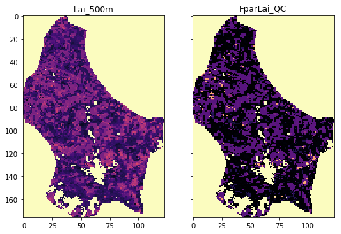
for i, the_layer in enumerate(["Lai_500m", "FparLai_QC"]):
data = mosaic_and_clip(tiles,
149,
2017,
folder="data/",
layer=the_layer,
shpfile="data/TM_WORLD_BORDERS-0.3.shp",
country_code="LU",
frmat="MEM")
axs[i].imshow(data, interpolation="nearest", vmin=0, vmax=120,
cmap=plt.cm.magma)
axs[i].set_title(the_layer)

# Testing GeoTIFF return arrays
tiles = ["h17v03", "h17v04", "h18v03", "h18v04"]
fig, axs = plt.subplots(nrows=1, ncols=2, sharex=True, sharey=True,
figsize=(8, 18))
for i, the_layer in enumerate(["Lai_500m", "FparLai_QC"]):
fname = mosaic_and_clip(tiles,
149,
2017,
folder="data/",
layer=the_layer,
shpfile="data/TM_WORLD_BORDERS-0.3.shp",
country_code="LU",
frmat="GTiff")
print(fname)
g = gdal.Open(fname)
data = g.ReadAsArray()
axs[i].imshow(data, interpolation="nearest", vmin=0, vmax=120,
cmap=plt.cm.magma)
axs[i].set_title(the_layer)
data/Lai_500m_2017_149_LU.tif
data/FparLai_QC_2017_149_LU.tif
So this appears to have worked… visually. A more thorough analysis would be required, possibly opening the files and checking that you can read out individual locations.
We now have an easy to call function that does a lot of complex processing behind the scenes to provide us with the actual data that we might want to use.
3.4.2.3 interpreting QA
We can now get the data describing LAI and QC for any given date (and country, given the limitations of the data in the system!)
The LAI dataset is decribed on the NASA page, with the bit field information given in the file spec
BITFIELDS
-------------
0,0 MODLAND_QC bits
'0' = Good Quality (main algorithm with or without saturation)
'1' = Other Quality (back-up algorithm or fill values)
1,1 SENSOR
'0' = Terra
'1' = Aqua
2,2 DEADDETECTOR
'0' = Detectors apparently fine for up to 50% of channels 1,2
'1' = Dead detectors caused >50% adjacent detector retrieval
3,4 CLOUDSTATE (this inherited from Aggregate_QC bits {0,1} cloud state)
'00' = 0 Significant clouds NOT present (clear)
'01' = 1 Significant clouds WERE present
'10' = 2 Mixed cloud present on pixel
'11' = 3 Cloud state not defined,assumed clear
5,7 SCF_QC (3-bit, (range '000'..100') 5 level Confidence Quality score.
'000' = 0, Main (RT) method used, best result possible (no saturation)
'001' = 1, Main (RT) method used with saturation. Good,very usable
'010' = 2, Main (RT) method failed due to bad geometry, empirical algorithm used
'011' = 3, Main (RT) method failed due to problems other than geometry,
empirical algorithm used
'100' = 4, Pixel not produced at all, value coudn't be retrieved
(possible reasons: bad L1B data, unusable MOD09GA data)
qa_data = mosaic_and_clip(tiles,
149,
2017,
layer="FparLai_QC")
print(f'Unique QA values found')
print(sorted(np.unique(qa_data)))
Unique QA values found
[0, 2, 8, 10, 16, 18, 32, 34, 40, 42, 48, 50, 97, 99, 105, 107, 113, 115, 157, 255]
We will use the bitfield SFC_QC as our main way to interpret
quality.
The information above tells us we need to extract bits 5-7 from the QA dataset.
Let’s be clear what we mean by this.
The dataset FparLai_QC is of data type uint8, unsigned 8-bit
integer (i.e. unsigned byte).
so, for example, in the file above, we see the following 19 unique codes:
import pandas as pd
# some pretty printing code using pandas
qas = np.array([[format(q,'3d'),format(q,'08b')] \
for q in sorted(np.unique(qa_data))]).T
pd.DataFrame({'decimal representation': qas[0],
'binary representation': qas[1]})
Recall the truth table for the and operation:
| A | B | A and B |
|---|---|---|
| T | T | T |
| T | F | F |
| F | T | F |
| F | F | F |
For binary rerpresentation, we replace True by 1 and False
by 0.
We also use the bitwise and operator &:
| A | B | A & B |
|---|---|---|
| 1 | 1 | 1 |
| 1 | 0 | 0 |
| 0 | 1 | 0 |
| 0 | 0 | 0 |
Notice that A & B only lets the value of B come through if A
is 1. Setting A as 0 effectively ‘switches off’ the
information in B.
We can see this more clearly using a combination of bits:
A = 0b01100
B = 0b11010
print('A =',format(A,'#07b'))
print('B =',format(B,'#07b'))
print('C = A & B =',format(A & B,'#07b'))
A = 0b01100
B = 0b11010
C = A & B = 0b01000
Here, the ‘mask’ A is set to 1 for bits 2 and 3 : 0b01100.
So only the information in bits 2 and 3 of B is passed through to
C. If we change the other bits in B, it has no effect on C:
A = 0b01100
B = 0b01001
print('A =',format(A,'#07b'))
print('B =',format(B,'#07b'))
print('C = A & B =',format(A & B,'#07b'))
A = 0b01100
B = 0b01001
C = A & B = 0b01000
Exercise 3.4.2
- copy the code from the block above
- change the bit values in
Band check that only the information in the bits set as1inAis passed through toC - make a new mask
Aand re-confirm your findings for this mask
Hint
We are using A as a mask, so we set the ‘pass’ bits in A to
1 and ‘block’ to 0
# do exercise here
So, to extract bits 5-7 (the 3 left-most bits) from an 8-bit number, we
first perform a bitwise (binary) ‘and’ operation with the mask
0b11100000. This has 5 0s to the right.
Because we have trailing zeros (to the right) of the masked value, we
perform a bit shift operation (>>) of length 5:
import pandas as pd
# some pretty printing code using pandas
mask = 0b11100000
unique_qa_data = sorted(np.unique(qa_data))
decimal = np.zeros_like(unique_qa_data, dtype=object)
binary = np.zeros_like(unique_qa_data, dtype=object)
masked = np.zeros_like(unique_qa_data, dtype=object)
shifted = np.zeros_like(unique_qa_data, dtype=object)
sfc_qc = np.zeros_like(unique_qa_data, dtype=object)
for i, q in enumerate(unique_qa_data):
decimal[i] = format(q, '3d')
binary[i] = format(q, '08b')
masked[i] = format ( (q & mask), '08b')
shifted[i] = format((q & mask)>>5, '08b')
sfc_qc[i] = format((q & mask)>>5, '03d')
pd.DataFrame({'decimal': decimal, 'binary': binary,
'masked': masked,'shifted': shifted,
'SFC_QC': sfc_qc})
Looking back at the data interpretation table:
5,7 SCF_QC (3-bit, (range '000'..100') 5 level Confidence Quality score.
'000' = 0, Main (RT) method used, best result possible (no saturation)
'001' = 1, Main (RT) method used with saturation. Good,very usable
'010' = 2, Main (RT) method failed due to bad geometry, empirical algorithm used
'011' = 3, Main (RT) method failed due to problems other than geometry,
empirical algorithm used
'100' = 4, Pixel not produced at all, value coudn't be retrieved
(possible reasons: bad L1B data, unusable MOD09GA data)
we can see that QA values of 0,2,,8,10,16 and 18 all correspond to
Main (RT) method used, best result possible (no saturation), values
of 32,34, 40, 42,48, 50 to
Main (RT) method used with saturation. Good,very usable etc.
We can apply this operation to the whole QA numpy array. While can use
the standard & and >> symbols, for array operations, the
functions np.bitwise_and and np.right_shift are preferred:
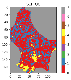
sfc_qa = np.right_shift(np.bitwise_and(qa_data, mask), 5)
plt.title('SCF_QC')
plt.imshow(sfc_qa,cmap=plt.cm.Set1)
plt.colorbar()
<matplotlib.colorbar.Colorbar at 0x12238d898>
Exercise 3.4.3
- For the momnent, assume that we only want data which have
SCF_QCset to0(i.e.Main (RT) method used, best result possible (no saturation)). - read in the LAI data associated with this dataset, and set unwanted
LAI data (i.e. those with
SCF_QCnot set to0) to Not a Number (np.nan) - plot the resultant dataset
Hint
Use the previous function to obtain the corresponding LAI dataset for the current date.
The LAI image plotted should show ‘white’ (no value) everywhere the
SCF_QC image above is not red.
# do exercise here
3.4.2.4 Deriving a weight from QA
What we want to develop here is a translation from the QA information
(given in FparLai_QC) to a weight that we can apply to the data.
If the quality is poor, we want a low weight. If the quality is good, a high weight. It makes sense to call the highest weight 1.0.
For LAI, we can use the QA information contained in bits 5-7 of
FparLai_QC to achieve this.
The valid codes for SCF_QC here are:
0 : Main (RT) method used best result possible (no saturation)
1 : Main (RT) method used with saturation. Good very usable
2 : Main (RT) method failed due to bad geometry empirical algorithm used
3 : Main (RT) method failed due to problems other than geometry empirical algorithm used
where we have translated the binary representations above to decimal.
A useful way of this to some weight is to define a real number
\(n\), where \(0 <= n < 1\) and raise this to the power of
SCF_QC.
So, for example is we set n = 0.61803398875 (the inverse golden
ratio):
n = 0.61803398875
for SCF_QC in [0,1,2,3]:
weight = n**SCF_QC
print(f'SCF_QC: {SCF_QC} => weight {weight:.4f}')
plt.plot(SCF_QC, weight, '*')
SCF_QC: 0 => weight 1.0000
SCF_QC: 1 => weight 0.6180
SCF_QC: 2 => weight 0.3820
SCF_QC: 3 => weight 0.2361
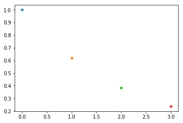
Then we have the following meaning for the weights:
1.0000 : Main (RT) method used best result possible (no saturation)
0.6180 : Main (RT) method used with saturation. Good very usable
0.3820 : Main (RT) method failed due to bad geometry empirical algorithm used
0.2361 : Main (RT) method failed due to problems other than geometry empirical algorithm used
Altghough we could vary the value of \(n\) used and get subtle variations, this sort of weighting should produce the desired result.
Exercise 3.4.4
- write a function that converts from
SCF_QCvalue to weight. - apply this to the
SCF_QCdataset we generated above. - display the weight image, along side the
SCF_QCand visually check you have the weighting correct
Hint
Since only [0,1,2,3] are valid inputs, you could use conditions such
as:
(SCF_QC == i) * (n ** i)
for valid values of i. This should then work correctly for arrays.
# do exercise here
The code you write can again be split into two very simple functions that you ought to test: One is just masking and shfting the QA data to obtain the SFC_QC flag on its own. A second part deals with calculating the weights depending on whether the SFC_QC flag has values of 0, 1, 2 or 3. For any other values, it ought to be 0.
def get_sfc_qc(qa_data, mask57 = 0b11100000):
sfc_qa = np.right_shift(np.bitwise_and(qa_data, mask57), 5)
return sfc_qa
def get_scaling(sfc_qa, golden_ratio=0.61803398875):
weight = np.zeros_like(sfc_qa, dtype=np.float)
for qa_val in [0, 1, 2, 3]:
weight[sfc_qa == qa_val] = np.power(golden_ratio, float(qa_val))
return weight
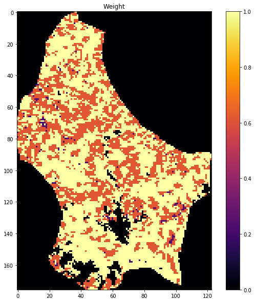
sfc_qa = get_sfc_qc(qa_data)
weights = get_scaling(sfc_qa)
plt.figure(figsize=(10,10))
plt.imshow(weights, vmin=0, vmax=1, interpolation="nearest",
cmap=plt.cm.inferno)
plt.colorbar()
plt.title("Weight")
Text(0.5, 1.0, 'Weight')
3.4.3 A time series
You should now know how to access and download datasets from the NASA servers and have developed functions to do this.
You should also know how to select a dataset from a set of hdf files, and mosaic, mask and crop the data to correspond to some vector boundary. This is a very common task in geospatial processing.
You should also know how to evaluate QA information and use this to determine some quality weight. This includes an understanding of how to interpret and use binary data fields in a QA dataset.
We now consider the case where we want to analyse a time series of data. We will use LAI over time to exemplify this.
We have already developed a file that returns an array (or a GeoTIFF)
for a given date above, called mosaic_and_clip. We can loop over
different dates while feeding the data into a so-called data
cube.
This is how you get the LAI
tiles = []
for h in [17, 18]:
for v in [3, 4]:
tiles.append(f"h{h:02d}v{v:02d}")
print(tiles)
year = 2017
doy = 149
data = mosaic_and_clip(tiles,
doy,
year,
folder="data/",
layer="Lai_500m",
shpfile="data/TM_WORLD_BORDERS-0.3.shp",
country_code="LU",
frmat="MEM")
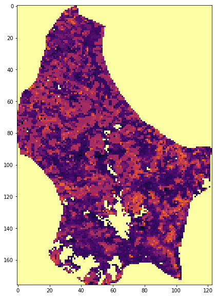
plt.figure(figsize=(10,10))
plt.imshow(data/10., vmin=0, vmax=10, interpolation="nearest",
cmap=plt.cm.inferno)
['h17v03', 'h17v04', 'h18v03', 'h18v04']
<matplotlib.image.AxesImage at 0x121e4c278>
Exercise 3.4.5
- Test that the code above works for reading the QA dataset as well.
- Write a function that reads both the LAI dataset and the QA data, scales the LAI data appropriately and produces a weight from the QA data.
- Return the LAI data and the weight
Hint
Scale LAI by multiplying by 0.1 as above.
# do exercise here
You should end up with something like:
def process_single_date(tiles,
doy,
year,
folder="data/",
shpfile="data/TM_WORLD_BORDERS-0.3.shp",
country_code="LU",
frmat="MEM"):
lai_data = mosaic_and_clip(tiles,
doy,
year,
folder=folder,
layer="Lai_500m",
shpfile=shpfile,
country_code=country_code,
frmat="MEM")*0.1
# Note the scaling!
qa_data = mosaic_and_clip(tiles,
doy,
year,
folder=folder,
layer="FparLai_QC",
shpfile=shpfile,
country_code=country_code,
frmat="MEM")
sfc_qa = get_sfc_qc(qa_data)
weights = get_scaling(sfc_qa)
return lai_data, weights
tiles = []
for h in [17, 18]:
for v in [3, 4]:
tiles.append(f"h{h:02d}v{v:02d}")
year = 2017
doy = 273
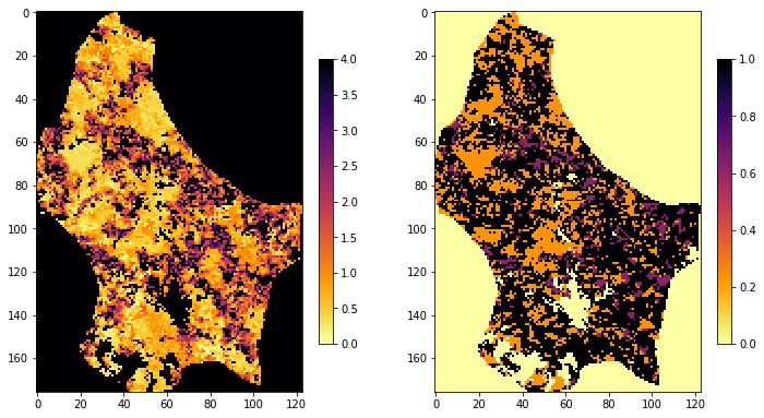
fig, axs = plt.subplots(nrows=1, ncols=2, figsize=(12, 24))
lai, weights = process_single_date(tiles,
doy,
year)
img1 = axs[0].imshow(lai, interpolation="nearest", vmin=0, vmax=4,
cmap=plt.cm.inferno_r)
img2 = axs[1].imshow(weights, interpolation="nearest", vmin=0,
cmap=plt.cm.inferno_r)
plt.colorbar(img1,ax=axs[0],shrink=0.2)
plt.colorbar(img2,ax=axs[1],shrink=0.2)
<matplotlib.colorbar.Colorbar at 0x1226e8c18>
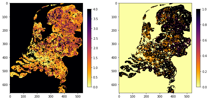
tiles = []
for h in [17, 18]:
for v in [3, 4]:
tiles.append(f"h{h:02d}v{v:02d}")
year = 2017
doy = 273
fig, axs = plt.subplots(nrows=1, ncols=2, figsize=(12, 24))
lai, weights = process_single_date(tiles,
doy,
year, country_code="NL")
img1 = axs[0].imshow(lai, interpolation="nearest", vmin=0, vmax=4,
cmap=plt.cm.inferno_r)
img2 = axs[1].imshow(weights, interpolation="nearest", vmin=0,
cmap=plt.cm.inferno_r)
plt.colorbar(img1,ax=axs[0],shrink=0.2)
plt.colorbar(img2,ax=axs[1],shrink=0.2)
<matplotlib.colorbar.Colorbar at 0x122b1ffd0>
Try it out:
Exercise 3.4.6
- Now we have some code to get the LAI and weight for one day, write a function that generates an annual dataset of LAI and weight
- show the dataset shapes
- Show the code works by plotting datasets for the beggining, middle and end of year
Hint
The result should be a set of two 3D numpy arrays
Really, all you need do is loop over each day, and add the new dataszet to a list.
Remember to create an initial empty list before you loop over day.
Think what might happen if the data for some day is missing.
# do exercise here
Although there are other ways of doing this, we can build up on what we had before, and just loop over days
from datetime import datetime, timedelta
def process_timeseries(year,
tiles,
folder,
shpfile,
country_code,
verbose=True):
today = datetime(year, 1, 1)
dates = []
for i in range(92):
if (i%10 == 0) and verbose:
print(f"Doing {str(today):s}")
if today.year != year:
break
doy = int(today.strftime("%j"))
this_lai, this_weight = process_single_date(
tiles,
doy,
year,
folder=folder,
shpfile=shpfile,
country_code=country_code,
frmat="MEM")
if doy == 1:
# First day, create outputs!
ny, nx = this_lai.shape
lai_array = np.zeros((ny, nx, 92))
weights_array = np.zeros((ny, nx, 92))
lai_array[:, :, i] = this_lai
weights_array[:, :, i] = this_weight
dates.append(today)
today = today + timedelta(days=4)
return dates, lai_array, weights_array
tiles = []
for h in [17, 18]:
for v in [3, 4]:
tiles.append(f"h{h:02d}v{v:02d}")
year = 2017
dates, lai_array, weights_array = process_timeseries(
year,
tiles,
folder="data/",
shpfile="data/TM_WORLD_BORDERS-0.3.shp",
country_code="NL")
Doing 2017-01-01 00:00:00
Doing 2017-02-10 00:00:00
Doing 2017-03-22 00:00:00
Doing 2017-05-01 00:00:00
Doing 2017-06-10 00:00:00
Doing 2017-07-20 00:00:00
Doing 2017-08-29 00:00:00
Doing 2017-10-08 00:00:00
Doing 2017-11-17 00:00:00
Doing 2017-12-27 00:00:00
fig, axs = plt.subplots(nrows=4, ncols=2, sharex=True,
sharey=True, figsize=(32, 24))
for i, tstep in enumerate([10, 30, 60, 80]):
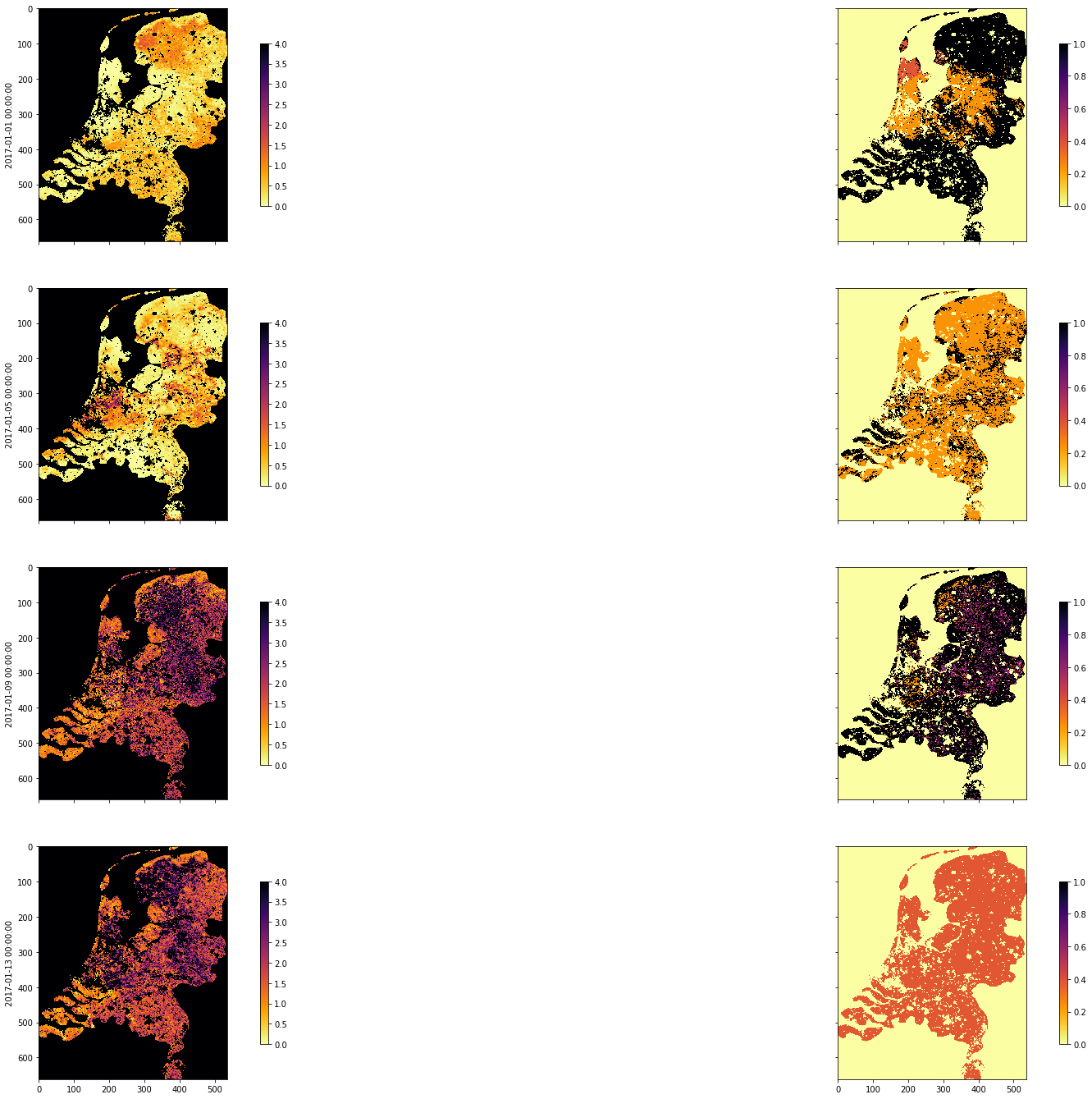
img1 = axs[i][0].imshow(lai_array[:, :, tstep],
interpolation="nearest", vmin=0, vmax=4,
cmap=plt.cm.inferno_r)
img2 = axs[i][1].imshow(weights_array[:, :, tstep],
interpolation="nearest", vmin=0, vmax=1,
cmap=plt.cm.inferno_r)
plt.colorbar(img1,ax=axs[i][0],shrink=0.7)
plt.colorbar(img2,ax=axs[i][1],shrink=0.7)
axs[i][0].set_ylabel(dates[i])
tiles = []
for h in [17, 18]:
for v in [3, 4]:
tiles.append(f"h{h:02d}v{v:02d}")
year = 2017
dates, lai_array, weights_array = process_timeseries(
year,
tiles,
folder="data/",
shpfile="data/TM_WORLD_BORDERS-0.3.shp",
country_code="BE")
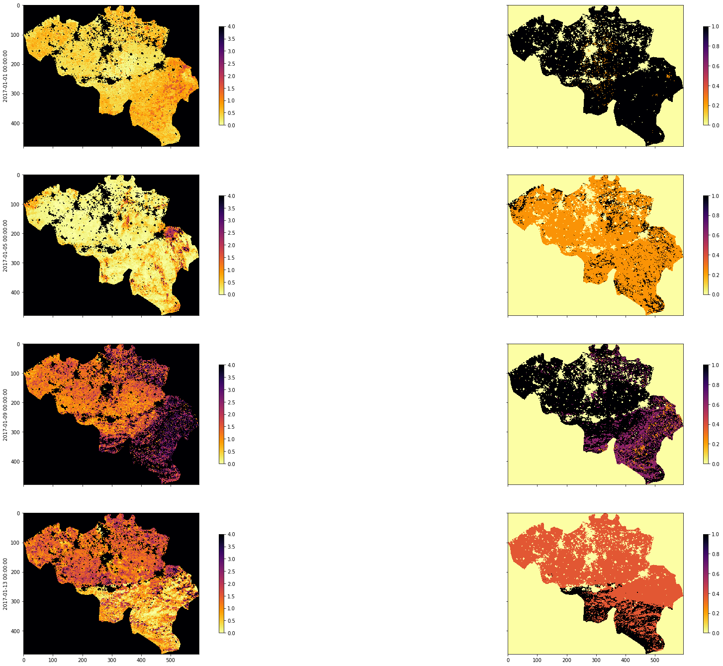
fig, axs = plt.subplots(
nrows=4, ncols=2, sharex=True, sharey=True, figsize=(32, 24))
for i, tstep in enumerate([10, 30, 60, 80]):
img1 = axs[i][0].imshow(
lai_array[:, :, tstep],
interpolation="nearest",
vmin=0,
vmax=4,
cmap=plt.cm.inferno_r)
img2 = axs[i][1].imshow(
weights_array[:, :, tstep],
interpolation="nearest",
vmin=0,
vmax=1,
cmap=plt.cm.inferno_r)
plt.colorbar(img1, ax=axs[i][0], shrink=0.7)
plt.colorbar(img2, ax=axs[i][1], shrink=0.7)
axs[i][0].set_ylabel(dates[i])
Doing 2017-01-01 00:00:00
Doing 2017-02-10 00:00:00
Doing 2017-03-22 00:00:00
Doing 2017-05-01 00:00:00
Doing 2017-06-10 00:00:00
Doing 2017-07-20 00:00:00
Doing 2017-08-29 00:00:00
Doing 2017-10-08 00:00:00
Doing 2017-11-17 00:00:00
Doing 2017-12-27 00:00:00
Now let’s read the data in:
3.4.4 Weighted interpolation
3.4.4.1 Smoothing
Some animations to help understand how we can use convolution to perform a weighted interpolation are given. You should got through these if you have not previously come across convolution filtering.
In convolution, we combine a signal \(y\) with a filter \(f\) to achieve a filtered signal. For example, if we have an noisy signal, we will attempt to reduce the influence of high frequency information in the signal (a ‘low pass’ filter, as we let the low frequency information pass).
We can perform a weighted interpolation by:
- numerator = smooth( signal \(\times\) weight)
- denominator = smooth( weight)
- result = numerator/denominator
sigma = 8
import scipy
import scipy.ndimage.filters
x = np.arange(-3*sigma,3*sigma+1)
gaussian = np.exp((-(x/sigma)**2)/2.0)
FIPS ='LU'
dates, lai_array, weights_array = process_timeseries( year, tiles, folder="data/",
shpfile="data/TM_WORLD_BORDERS-0.3.shp", country_code=FIPS)
print(lai_array.shape, weights_array.shape) #Check the output array shapes
numerator = scipy.ndimage.filters.convolve1d(lai_array * weights_array, gaussian, axis=2,mode='wrap')
denominator = scipy.ndimage.filters.convolve1d(weights_array, gaussian, axis=2,mode='wrap')
# avoid divide by 0 problems by setting zero values
# of the denominator to not a number (NaN)
denominator[denominator==0] = np.nan
interpolated_lai = numerator/denominator
print(interpolated_lai.shape)
Doing 2017-01-01 00:00:00
Doing 2017-02-10 00:00:00
Doing 2017-03-22 00:00:00
Doing 2017-05-01 00:00:00
Doing 2017-06-10 00:00:00
Doing 2017-07-20 00:00:00
Doing 2017-08-29 00:00:00
Doing 2017-10-08 00:00:00
Doing 2017-11-17 00:00:00
Doing 2017-12-27 00:00:00
(176, 123, 92) (176, 123, 92)
(176, 123, 92)
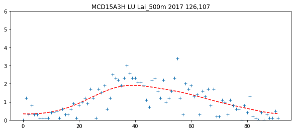
## find where the weight is highest, and lets look there!
sweight = weights_array.sum(axis=2)
r,c = np.where(sweight == np.max(sweight))
plt.figure(figsize=(10,4))
plt.title(f'{product} {FIPS} {params[0]} {year} {r[0]},{c[0]}')
ipixel = 0 # To plot the i-th pixel
plt.plot((interpolated_lai)[r[ipixel],c[ipixel],:],'r--')
plt.plot((lai_array)[r[ipixel],c[ipixel],:],'+')
plt.ylim(0,6)
(0, 6)
Exercise 3.4.7
- select some pixels (row, col) from the lai dataset and plot the original LAI, the interpolated LAI, and the weight
# do exercise here
3.4.5 Making movies
It is often useful to animate time series information. There are several ways of doing this.
Bear in mind that the larger the datasets, number of images and/or frames, the more time it is likely to take to generate the animations. You probably don’t want more than around 100 frames to make an animation of this sort.
The two approaches we will use are:
- Javascript HTML in the notebook using
anim.to_jshtml()frommatplotlib.animation - Animated gif using the
imageiolibrary
3.4.5.1 Javascript HTML
This approach uses javascript in html within the notebook to genrate an animation and player. The player is useful, in that we can easily stop at and explore individual frames.
The HTML representation is written to a temporary directory (internally to anim.to_jshtml()) but deleted on exit.
from matplotlib import animation
import matplotlib.pylab as plt
from IPython.display import HTML
'''
lai movie javascript/html (jshtml)
'''
#fig, ax = plt.subplots(figsize=(10,10))
fig = plt.figure(0,figsize=(10,10))
# define an animate function
# with the argument i, the frame number
def animate(i):
# show frame i of the ilai dataset
plt.figure(0)
im = plt.imshow(interpolated_lai[:,:,i],vmin=0,vmax=6,cmap=plt.cm.inferno_r)
plt.title(f'{product} {FIPS} {params[0]} {year} DOY {4*i+1:03d}')
# make sure to return a tuple!!
return (im,)
# set up the animation
anim = animation.FuncAnimation(fig, animate,
frames=interpolated_lai.shape[2], interval=40,
blit=True)
# display animation as HTML
HTML(anim.to_jshtml())
3.4.5.2 Animated gif
In the second approach, we save individual frames of an animation, and
read them in, using imageio.imread() into a list. We choose to write
the individual frames here to a temporary directory (so they are cleaned
up on exit).
This list of imageio datasets is then fed to
`imageio.mimsave() <https://imageio.readthedocs.io/en/stable/userapi.html>`__
to save the sequence as an animated gif. This can then be displayed in a
notebook cell (or otherwise). Note that the file
data/MCD15A3H.A2017.h1_78_v0_34_LU.006.gif
is saved in this case.
import imageio
import tempfile
from pathlib import Path
'''
lai movie as animated gif
'''
# switch interactive plotting off
# as we just want to save the frames,
# not plot them now
plt.ioff()
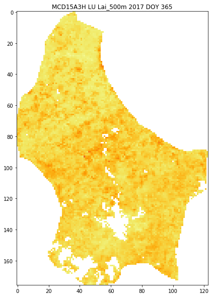
allopfile = Path('images', f'{product}_{FIPS}_{params[0]}_{year}_DOY{4*i+1:03d}')
#get_filename(FIPS,year,doy,tile,destination_folder='images')
images = []
with tempfile.TemporaryDirectory() as tmpdirname:
ofile = f'{tmpdirname}/tmp.png'
for i in range(interpolated_lai.shape[2]):
plt.figure(0,figsize=(10,10))
# don' display the interim frames
plt.ioff()
plt.clf()
plt.imshow(interpolated_lai[:,:,i],vmin=0,vmax=6,cmap=plt.cm.inferno_r)
plt.title(f'{product} {FIPS} {params[0]} {year} DOY {4*i+1:03d}')
plt.colorbar(shrink=0.85)
plt.savefig(ofile)
images.append(imageio.imread(ofile))
plt.clf()
imageio.mimsave(f'{allopfile}.gif', images)
print(f'{allopfile}.gif')
# switch interactive plotting back on
plt.ion()
images/MCD15A3H_LU_Lai_500m_2017_DOY365.gif
<Figure size 720x720 with 0 Axes>

Exercise 3.4.8
- Write a set of functions, with clear commenting and document strings
tha:
- develops the LAI and QA dataset for a given year to produce LAI data and weight
- produces interpolated / smoothed LAI data as a numpy 3D array for the year
- saves the resultant numpy dataset in a
npzfile
- Once y
Hint
Put all of the material above together.
Remember np.savez()!
# do exercise here