# All imports go here. Run me first!
import datetime
from pathlib import Path  # Checks for files and so on
import numpy as np  # Numpy for arrays and so on
import pandas as pd
import sys
import matplotlib.pyplot as plt  # Matplotlib for plotting
# Ensure the plots are shown in the notebook
%matplotlib inline

import gdal
import osr
import numpy as np

from geog0111.geog_data import procure_dataset

if not Path("data/mod14_data").exists():
    _ = procure_dataset("mod14_data", destination_folder="data/mod14_data")
else:
    print("Data already available")
Data already available
Group project: Fire and teleconnections
There is much public and scientific interest in monitoring and predicting the activity of wildfires and such topics are often in the media, or here for a more recent event.
Part of this interest stems from the role fire plays in issues such as land cover change, deforestation and forest degradation and Carbon emissions from the land surface to the atmosphere, but also of concern are human health impacts, effects on soil, erosion, etc. The impacts of fire should not however be considered as wholy negative, as it plays a significant role in natural ecosystem processes.
For many regions of the Earth, there are large inter-annual variations in the timing, frequency and severity of wildfires. Whilst anthropogenic activity accounts for a large proportion of fires started, this is not in itself a new phenomenon, and fire has been and is used by humans to manage their environment.
Fires spread where: (i) there is an ignition source (lightning or man, mostly); (ii) sufficient combustible fuel to maintain the fire. The latter is strongly dependent on fuel loads and mositure content, as well as meteorological conditions. Generally then, when conditions are drier (and there is sufficient fuel and appropriate weather conditions), we would expect fire spread to increase. If the number of ignitions remained approximately constant, this would mean more fires. Many models of fire activity predict increases in fire frequency in the coming decades, although there may well be different behaviours in different parts of the world.

Satellite data has been able to provide us with increasingly useful tools for monitoring wildfire activity, particularly since 2000 with the MODIS instruments on the NASA Terra and Aqua (2002) satellites. A suite of ‘fire’ products have been generated from these data that have been used in a large number of publications and practical/management projects.
There is growing evidence of ‘teleconnection’ links between fire occurence and large scale climate patterns, such as ENSO.

The proposed mechanisms are essentially that such climatic patterns are linked to local water status and temperature and thus affect the ability of fires to spread. For some regions of the Earth, empirical models built from such considerations have quite reasonable predictive skill, meaning that fire season severity might be predicted some months ahead of time.
In this Session..
In this session, you will be working in groups (of 3 or 4) to build a computer code in Python to explore links between fire activity and Sea Surface Temperature anomalies.
This is a team exercise, but does not form part of your formal assessment for this course. You should be able to complete the exercise in a 3-4 hour session, if you work effectively as a team. Staff will be on hand to provide pointers.
You should be able to complete the exercise using coding skills and python modules that you have previously experience of, though we will also provide some pointers to get you started.
In a nutshell, the goal of this exercise is
Using monthly fire count data from MODIS Terra, develop and test a predictive model for the number of fires per unit area per year driven by Sea Surface Temperature anomaly data.
The datasets should be created at 5 degree resolution on a latitude/longitude grid, as climate patterns will probably show some sort of response at broader spatial scales.
You should concentrate on building the model that predicts peak fire count in a particular year at a particular location, i.e. derive your model for annual peak fire count.
Datasets
We suggest that the datasets you use of this analysis, following Chen at al. (2011), are:
- MODIS Terra fire counts (2001-2011) (MOD14CMH). The particular dataset you will want from the file is ‘SUBDATASET_2 [360x720] CloudCorrFirePix (16-bit integer)’.
- Climate index data from NOAA (e.g. see this list)
If you ever wish to take this study further, you can find various other useful datasets such as these.
Fire Data
The MOD14CMH CMG data are available from the UMD ftp server but have also been packaged for you and can be imported using the following code (this has already been done in the first imports cell above):
from geog0111.geog_data import procure_dataset

_ = procure_dataset("mod14_data",
                destination_folder="data/mod14_data")
The data are in HDF format, and you ought to be able to read them nto numpy arrays an operate with them. Note that there is data for MODIS TERRA and AQUA sensors, and if you want to use them together, you need to figure out the overlap period (AQUA only started providing data halfway through 2002).
The teleconnections data
Teleconnections data are available from a large number of places on the internet. You can find some sources of inspiration here. The data can be processed in two different ways: either as it is, or as anomalies (where you define a baseline temporal period, calculate some average value, and look at the residual between the actual index and the historical average). It’s up to you what index you may want to use, and whether you want to use anomalies or directly the index value.
The predictive model
The model is very simple: we assume that the there is a linear
relationship between the teleconnection at some given lag, and the
recorded number of thermal anomalies. Bear in mind that the aim is to
predict fire counts some months in advance using a teleconnection.
As pseudo-code, for a pixel location i,j, you’d have something like
this:
i, j # this is the pixel value
# Read in the peak fire month
peak_fire_month = get_peak_fire_month(i, j)
# Read in peak fire counts for all years for the pixel of interest
y = get_all_fire_counts_for_all_years(i, j)
# Loop over some lags
for lag in 0, ..., 12
do
    # Get the lagged teleconnection
    x = get_teleconnection_for_all_years(peak_fire_month - lag)
    # Perform linear regression and store the results
    m[lag], c[lag], r2[lag] = linear_regression(x, y)
done
best_lag = argmax(r2) # Select best lag
store_model(i, j, best_lag, m[best_lag], c[best_lag], r2[best_lag])
Splitting the tasks
You may want to assign tasks to individual members of the group. A reasonable split might be
- One person is responsible for the satellite data. This includes creating a 5 degree global resolution monthly dataset, and from it, derive for each grid cell, a peak fire month dataset, as well as a dataset with the fire counts at each peak fire month for all available years (more hints below)
- Another person might be in charge for getting hold of the teleconnections dataset, and process it into a suitable array
- Finally, some other person could be in charge of combining both fire counts and teleconnections datasets together and developing and testing a linear model to predict fire counts.
The satellite fire counts data
- The satellite data need to be aggregated to a coarser resolution of 5 degrees. This means that you have to sum the fire counts for every 10x10 original pixels, discarding missing values and so on. You ought to discard 2000 as there are only two months of data available for that year.
- A reasonable data model for this is a numpy array of size
n_months*n_years, nn, mm. You may also want to store the months and years as a 2D array (e.g.n_months*n_years,2) - Once you have this, you can loop over your fire array, selecting all
the fire counts for each year (e.g. 12 numbers) for each pixel, and
finding the location of the maximum (using e.g.
np.argmax). You’ll end up with an array of sizen_years, nn, mm. - So now you need to decide which month is, on average, the peak fire month. How could you do this? The mean is problematic, as you may end up with something like e.g. 6.5. Are there other statistical metrics that might results useful (e.g. see this)?
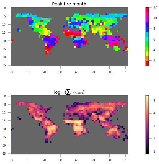
At this point, you should end up with one main array of size nn, mm
(e.g. 36, 72), where every grid cell is populated by the peak fire
number defined from the data, as well as the n_years,nn,nn array
with the fire counts at peak fire month. Make sure it is clear what you
mean by month number!!! Note that we also have data available for the
AQUA platform, and you may want to use it too.
If you plot them, they should look like this:
The teleconnections
- You can start with one teleconnection, but you may want to explore others.
- A data structure for the telecon data that might be useful and convenient is to stack two consecutive years together. It then makes it easy to loop over different lags (e.g. if your peak fire month for a pixel is February, then examining the 12 previous months can be done by looking at positions 13 (Feb), 12 (Jan), 11 (Dec previous year) and so on.
With this in mind, you should aim to have an array with your
teleconnection (or a dictionary of teleconnections!) with size
n_years*24.
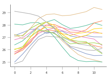
You can use the ESRL NOAA webpage to plot time series of your index (… indices) of choice, and make sure you have processed the data correctly.
Developing the model
The model is a simple linear model that relates the teleconnection value at some lag \(l\) with respect to the peak fire month (\(tc_{l}\)) with the number of fire counts for a given cell, \(N_{counts,\,i,j}\)
- You have to split the data into a testing and training set: select a number of years to fit the model, and another one to test the model.
- The training will produce estimates of the slope \(m\) and intercept \(c\) for every pixel and time lag \(l\).
- There are different ways to select the best lag, but the simplest one could be in terms of the coefficient of determination \(r^2\): just choose the highest!
- You should store the per grid cell model parameters, as well as probably the \(r^2\) (why?), and the optimal lag.
You can see an example of how this works on a particular grid cell in the following plot
Solution: getting the data
Getting the data needs the completion of a few stages:
- Searching for all the MODIS fire counts files
- Opening & reading each file, filtering the ocean grid cells
(indicated by
-1) - Aggregate the data to the coarser grid
- Create a 3D stack for all the months since the beggining of the time series.
- Find the peak month
These functionality has been implemented in
`geog0111/fire_practical_satellite.py <geog0111/fire_practical_satellite.py>`__,
where a bunch of functions are defined. Here are the headings of those
functions:
def get_mod14(folder="data/mod14_data", skip_files=2):
    """Gets hold of the MOD14 data. We can skip a couple of files
    from 2000, and just read in the data from 2001 to 2016.

    Parameters
    -----------
    folder: str
        The folder where the files are all located
    skip_files: int
        Number of files to skip at the start of the time series

    Returns
    -------
    REturns a list of pathlib objects with all the MOD14CMH HDF files
    """

def subsample_data(data, size=10, aggr=np.sum):
    """Subsample a 2D dataset by aggregating. Assumes that the input
    image or dataset will be aggregated over chunks of `size`
    by `size` pixels. You can select what aggregation method you
    want to use.

    Parameters
    -----------
    data: ndarray
        A 2D array of fire counts (for example)
    size: int
        The size of the aggregation in pixels. Identical for x and y
    aggr: function
        A function to perform the aggregation. By default, sum

    Returns
    ---------
    A downsampled and aggregated dataset
    """

def read_mod14_data(fich, layer=1):
    """Read the MOD14 data. Uses first layer by default.

    Parameters
    -----------
    fich: str
        A MOD14 HDF file
    layer: int
       The layer in the HDF file.

    Result
    -------
    Returns the data. Pixels with values <0 are set to 0.
    """


def create_subsampled_dataset():
    """Creates a subsampled datasets and extracts the dates.

    Returns
    --------
    Returns two arrays: a dates array (2 columns, years and months), as well
    as a 3D array of months*years, nx, ny cells.
    """
create_subsampled_dataset is in charge of creating the subsampled
dataset. It does so by calling get_mod14 which provides a list of
all the files, each file can then read into numpy arrays using GDAL in
read_mod14_data. The individual months can be subsampled by
subsample_data. This structure is very efficient: you can just loop
over the filenames that are returned by get_mod14, and then read and
aggregate before stacking the result.
Once the result is stacked, we can proceed grid by grid to find the peak
fire month. Since the peak fire actiivity month might change from year
to year, so perhaps using the “most popular value” (e.g the mode) is the
best approach. Additionally, we need to store the number of fires for
the peak month for all the years. This is done in
find_peak_and_fires.
Solution: getting hold of the teleconnection data
This is implemented in a single function in
`geog0111/fire_practical_telecon.py <geog0111/fire_practical_telecon.py>`__.
We can observe that in the NOAA site, a bunch of teleconnections are
available. They are all under the same URL, and have the same format.
The format is plain ASCII, with some headers, as well as a “footer” at
the end. Missing data are usually encoded by -9999, and each row in the
file contains the index for one year, each column storing one month.
We have satellite data from 2001 onwards, so we need teleconections from
2000 (to cover the previous year). The code produces a n_years, 24
array for easy indexing.
def get_telecon_data(
    telecon="nina34.data",
    dest_folder="data/mod14_data/",
    base_url="https://www.esrl.noaa.gov/psd/data/correlation/",
    start_year=2000,
    end_year=2016,
):
    """Downloads and processes the telenconnection data for easy
    model development. It returns a 2D array, where each row
    has 24 elements: element 12 is the teleconnection for January
    of the relevant year, and elements 0 to 11 are the teleconnection
    values for the months of the previous year.

    Parameters
    ------------
    telecon: str
        The name of the teleconnection. You can look it up from
        [this page](https://www.esrl.noaa.gov/psd/data/climateindices/list/)
    dest_folder: str
        The destination folder. It'll save the teleconnection there
    base_url: str
        The base URL for the NOAA server
    start_year: int
        The start year ;-)
    end_year: int
        The end year

    Returns
    ---------
    A 2D array with the teleconnection.
    """
Solution: the model fitting part
Once the teleconnection, fire peak month and fire counts for different
years are available, we can proceed to fit the model on a grid cell by
grid cell basis. The code that does this is available on
`geog0111/fire_practical_model.py <geog0111/fire_practical_model.py>`__
and looks like this:
for i in range(nn):
    for j in range(mm):
        # Now doing grid cell i, j
        # Get the peak fire activity month, and subtract one
        pf_month = peak_fire_month[i, j] - 1  # 1-based month
        # Get the fire counts for all training years
        counts = fire_count_year[:train_years, i, j]
        # The list comprehension sweeps over the telecon,
        # starting on peak fire month and going back 12 months
        reg = [
            scipy.stats.linregress(
                telecon[:train_years, pf_month - lager], counts
            )
            for lager in range(0, -12, -1)
        ]
        # Find the lag with the highest r^2
        iloc = np.argmax([x.rvalue ** 2 for x in reg])
        # etc
from geog0111.fire_practical_model import *
from geog0111.fire_practical_satellite import *
from geog0111.fire_practical_telecon import *

telecon = get_telecon_data()
mod14_dates, mod14_data = create_subsampled_dataset()
peak_fire_month, fire_count_year = find_peak_and_fires(mod14_dates, mod14_data)
slope, intercept, best_r2, best_lag = fit_model(
    telecon, peak_fire_month, fire_count_year, train_years=12)
plt.plot(telecon[:, 12:].T, '-')
[<matplotlib.lines.Line2D at 0x7fb3ceb25d30>,
 <matplotlib.lines.Line2D at 0x7fb3ceb25e80>,
 <matplotlib.lines.Line2D at 0x7fb3ceb25fd0>,
 <matplotlib.lines.Line2D at 0x7fb3ceb31160>,
 <matplotlib.lines.Line2D at 0x7fb3ceb312b0>,
 <matplotlib.lines.Line2D at 0x7fb3ceb31400>,
 <matplotlib.lines.Line2D at 0x7fb3ceb31550>,
 <matplotlib.lines.Line2D at 0x7fb3ceb316a0>,
 <matplotlib.lines.Line2D at 0x7fb3cf3a5a20>,
 <matplotlib.lines.Line2D at 0x7fb3ceb31908>,
 <matplotlib.lines.Line2D at 0x7fb3ceb31a58>,
 <matplotlib.lines.Line2D at 0x7fb3ceb31ba8>,
 <matplotlib.lines.Line2D at 0x7fb3ceb31cf8>,
 <matplotlib.lines.Line2D at 0x7fb3ceb31e48>,
 <matplotlib.lines.Line2D at 0x7fb3ceb31f98>,
 <matplotlib.lines.Line2D at 0x7fb3ceb38128>]
/home/ucfajlg/miniconda3/envs/python3/lib/python3.6/site-packages/matplotlib/font_manager.py:1328: UserWarning: findfont: Font family ['sans-serif'] not found. Falling back to DejaVu Sans
  (prop.get_family(), self.defaultFamily[fontext]))
fig, axs = plt.subplots(nrows=2, ncols=1, figsize=(21,9))
cmap = plt.cm.get_cmap("hsv", 12)
cmap.set_under("0.4")
im = axs[0].imshow(peak_fire_month, interpolation="nearest", vmin=1, vmax=12,cmap=cmap)
plt.colorbar(im, ax=axs[0], fraction=0.6)
axs[0].set_title("Peak fire month")

cmap = plt.cm.magma
cmap.set_bad('0.4')
im = axs[1].imshow(np.log10(fire_count_year.sum(axis=0)),
                   interpolation="nearest", cmap=cmap)
plt.colorbar(im, ax=axs[1], fraction=0.6)
axs[1].set_title(r"$\log_{10}(\sum F_{counts})$")
/home/ucfajlg/miniconda3/envs/python3/lib/python3.6/site-packages/ipykernel_launcher.py:10: RuntimeWarning: divide by zero encountered in log10
  # Remove the CWD from sys.path while we load stuff.
Text(0.5,1,'$\log_{10}(\sum F_{counts})$')
/home/ucfajlg/miniconda3/envs/python3/lib/python3.6/site-packages/matplotlib/font_manager.py:1328: UserWarning: findfont: Font family ['sans-serif'] not found. Falling back to DejaVu Sans
  (prop.get_family(), self.defaultFamily[fontext]))
fig, axs = plt.subplots(nrows=2, ncols=1, figsize=(31,12))
cmap = plt.cm.get_cmap("hsv", 12)
cmap.set_under("0.4")
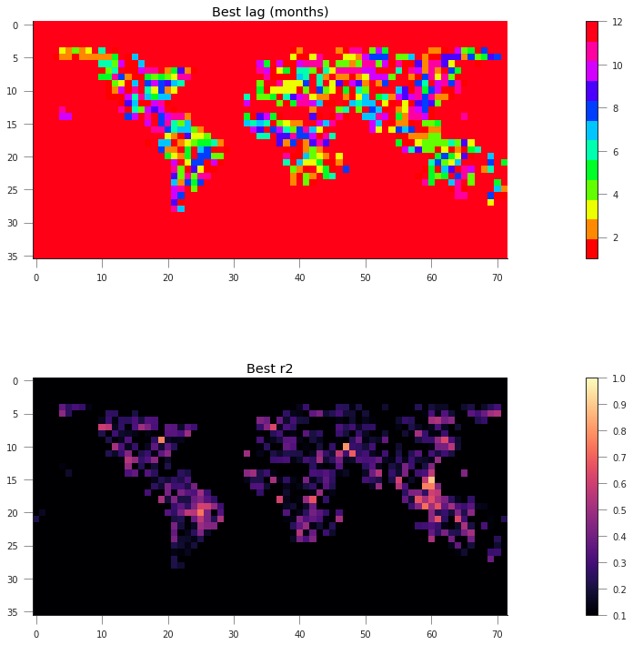
im = axs[0].imshow(best_lag, interpolation="nearest", vmin=1, vmax=12,cmap=cmap)
plt.colorbar(im, ax=axs[0], fraction=0.6)
axs[0].set_title("Best lag (months)")
cmap = plt.cm.magma
cmap.set_bad('0.4')
im = axs[1].imshow(best_r2,
interpolation="nearest", vmin=0.1, vmax=1,
cmap=cmap)
plt.colorbar(im, ax=axs[1], fraction=0.6)
axs[1].set_title("Best r2")
Text(0.5,1,'Best r2')
/home/ucfajlg/miniconda3/envs/python3/lib/python3.6/site-packages/matplotlib/font_manager.py:1328: UserWarning: findfont: Font family ['sans-serif'] not found. Falling back to DejaVu Sans
  (prop.get_family(), self.defaultFamily[fontext]))
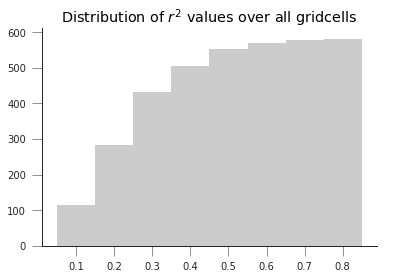
plt.hist(best_r2[best_r2 >= 0.1], bins=np.arange(0.1, 1, 0.1)-0.05, cumulative=True, histtype="stepfilled",
        color="0.8")
plt.title("Distribution of $r^2$ values over all gridcells")
Text(0.5,1,'Distribution of $r^2$ values over all gridcells')
/home/ucfajlg/miniconda3/envs/python3/lib/python3.6/site-packages/matplotlib/font_manager.py:1328: UserWarning: findfont: Font family ['sans-serif'] not found. Falling back to DejaVu Sans
  (prop.get_family(), self.defaultFamily[fontext]))
sensible_grids = best_r2 >= 0.1
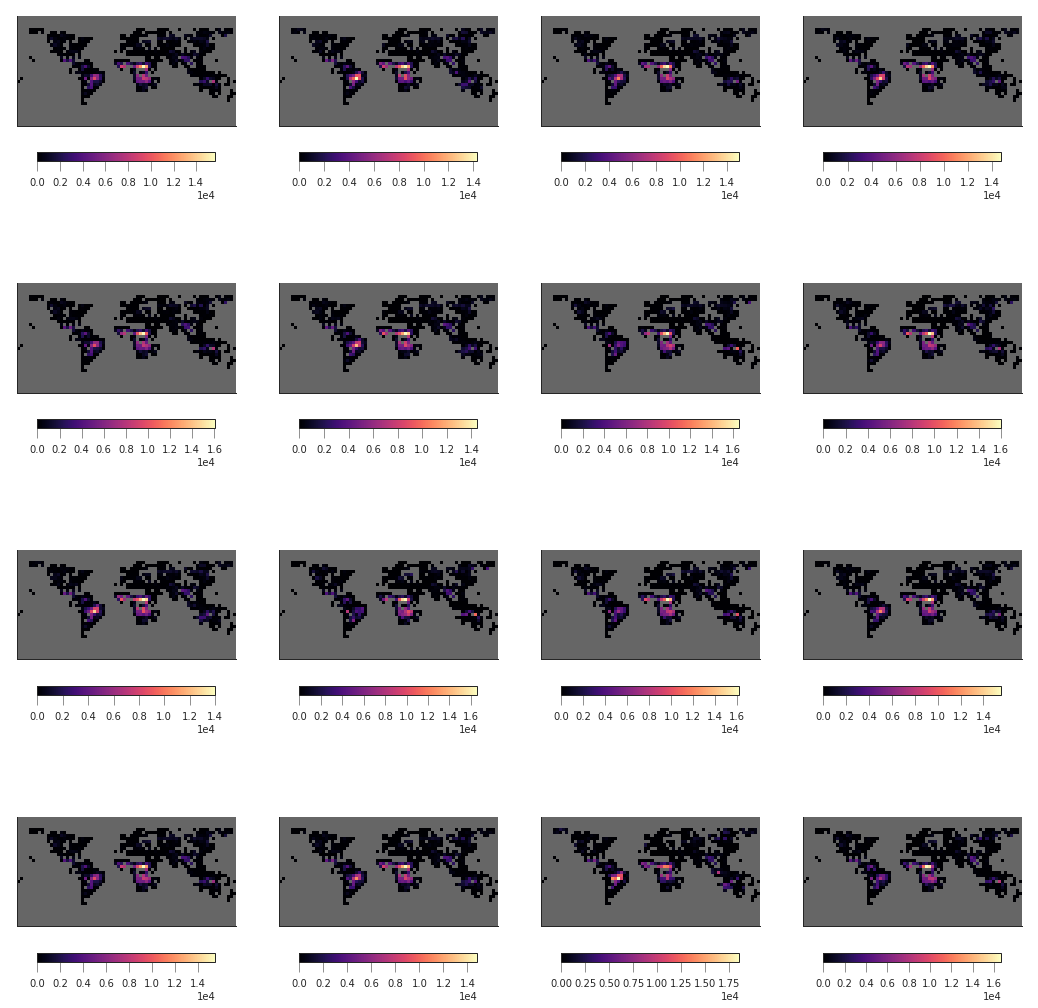
predicted_fire_counts = np.ones((16, 36, 72))*np.nan
fig, axs = plt.subplots(nrows=4, ncols=4, sharex=True, sharey=True,
figsize=(18, 18))
axs = axs.flatten()
for year in range(16):
x = telecon[year, :][11 + peak_fire_month]
y = slope*x + intercept
predicted_fire_counts[year, sensible_grids] = y[sensible_grids]
im=axs[year].imshow(predicted_fire_counts[year], interpolation="nearest",
vmin=0, cmap=plt.cm.magma)
axs[year].set_xticks([])
axs[year].set_yticks([])
plt.colorbar(im, ax=axs[year], fraction=0.05, orientation="horizontal")
/home/ucfajlg/miniconda3/envs/python3/lib/python3.6/site-packages/matplotlib/font_manager.py:1328: UserWarning: findfont: Font family ['sans-serif'] not found. Falling back to DejaVu Sans
  (prop.get_family(), self.defaultFamily[fontext]))
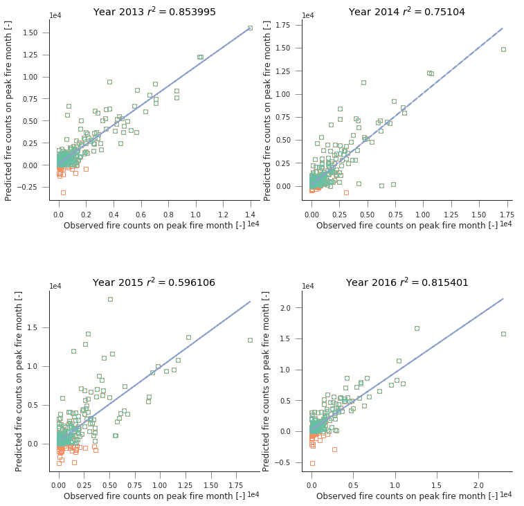
fig, axs = plt.subplots(nrows=2, ncols=2, figsize=(12,12))
axs = axs.flatten()
for i,year in enumerate(range(12, 16)):
    x = fire_count_year[year]
    y = predicted_fire_counts[year]
    axs[i].plot(x[sensible_grids], y[sensible_grids], 's', mfc="none")
    axs[i].plot(x[sensible_grids*(y>0)], y[sensible_grids*(y>0)], 'o', mfc="none")


    reg = scipy.stats.linregress(x[sensible_grids*(y>0)], y[sensible_grids*(y>0)])
    axs[i].plot(x[sensible_grids*(y>0)],
                x[sensible_grids*(y>0)]*reg.slope + reg.intercept, '--')
    axs[i].set_title(f"Year {2001+year:d} " + "$r^2=%g$"%reg.rvalue**2)
    axs[i].set_xlabel("Observed fire counts on peak fire month [-]")
    axs[i].set_ylabel("Predicted fire counts on peak fire month [-]")
/home/ucfajlg/miniconda3/envs/python3/lib/python3.6/site-packages/ipykernel_launcher.py:7: RuntimeWarning: invalid value encountered in greater
  import sys
/home/ucfajlg/miniconda3/envs/python3/lib/python3.6/site-packages/ipykernel_launcher.py:10: RuntimeWarning: invalid value encountered in greater
  # Remove the CWD from sys.path while we load stuff.
/home/ucfajlg/miniconda3/envs/python3/lib/python3.6/site-packages/ipykernel_launcher.py:11: RuntimeWarning: invalid value encountered in greater
  # This is added back by InteractiveShellApp.init_path()
/home/ucfajlg/miniconda3/envs/python3/lib/python3.6/site-packages/ipykernel_launcher.py:12: RuntimeWarning: invalid value encountered in greater
  if sys.path[0] == '':
/home/ucfajlg/miniconda3/envs/python3/lib/python3.6/site-packages/matplotlib/font_manager.py:1328: UserWarning: findfont: Font family ['sans-serif'] not found. Falling back to DejaVu Sans
  (prop.get_family(), self.defaultFamily[fontext]))