3.3 GDAL, and OGR masking
Table of Contents
3.3 GDAL, and OGR masking
3.3.1 The MODIS LAI data
3.3.1.1 try … except …
3.3.1.2 Get data
3.3.1.3 File Naming Convention
3.3.1.2 Dataset Naming Convention
3.3.2 MODIS dataset access
3.3.2.1 gdal.ReadAsArray()
3.3.2.2 Metadata
3.3.3 Reading and displaying data
3.3.3.1 glob
3.3.3.2 reading and displaying image data
3.3.3.3 subplot plotting
3.3.3.3 tile stitching
3.3.3.4 gdal virtual file
3.3.4 The country borders dataset
In this section, we’ll look at combining both raster and vector data to provide a masked dataset ready to use. We will produce a combined dataset of leaf area index (LAI) over the UK derived from the MODIS sensor. The MODIS LAI product is produced every 4 days and it is provided spatially tiled. Each tile covers around 1200 km x 1200 km of the Earth’s surface. Below you can see a map showing the MODIS tiling convention.
3.3.1 The MODIS LAI data
Let’s first test your NASA login:
import geog0111.nasa_requests as nasa_requests
from geog0111.cylog import cylog
%matplotlib inline

url = 'https://e4ftl01.cr.usgs.gov/MOTA/MCD15A3H.006/2018.09.30/'

# grab the HTML information
try:
    html = nasa_requests.get(url).text
    # test a few lines of the html
    if html[:20] == '<!DOCTYPE HTML PUBLI':
        print('this seems to be ok ... ')
        print('use cylog().login() anywhere you need to specify the tuple (username,password)')
except:
    print('login error ... try entering your username password again')
    print('then re-run this cell until it works')
    cylog(init=True)
this seems to be ok ...
use cylog().login() anywhere you need to specify the tuple (username,password)
3.3.1.1 try ... except ...
Note that we have used a try ... except structure above to trap any
errors.
import sys
try:
    # variable stupid not set
    print("I'm trying this but it will fail",stupid)
except NameError:
    '''
    trap the error
    (and ideally define some sensible behaviour)
    '''
    print("unset variable:",sys.exc_info()[1])
except:
    print("In case of other errors")
    print(sys.exc_info())
    # raise our own exception
    raise Exception('bad code')
unset variable: name 'stupid' is not defined
Generally, you should try to foresee the types of error you might generate, and provide specific traps for these so youy can control the code better.
In the case above, we allow the code execution to continue with a
NameError, but raise a further exception in case of any other
errors.
sys.exc_info() provides a tuple of information on what happened.
Exercise
- Write some code using
try ... exceptto trap aZeroDivisionError - provide a sensible result in such a case
hint
If you divide by zero, the result will be infinity, which is often not
what you want to happen. Instead, try dividing by a small number, such
as that provided by sys.float_info.epsilon.
# do exercise here
3.3.1.2 Get data
You should by now be able to download MODIS data, but in this case, the
data are provided (or downloaded for you) in the data folder as
files MCD15A3H.A2018273.h17v03.006.2018278143630.hdf and
MCD15A3H.A2018273.h18v03.006.2018278143633.hdf (and some files
*v04*hdf we will need later) by running the code below.
from geog0111.geog_data import *

filenames = ['MCD15A3H.A2018273.h17v03.006.2018278143630.hdf', \
            'MCD15A3H.A2018273.h18v03.006.2018278143633.hdf',\
            'MCD15A3H.A2018273.h17v04.006.2018278143630.hdf',\
            'MCD15A3H.A2018273.h18v04.006.2018278143638.hdf']
destination_folder="data"

for file_name in filenames:
    f = procure_dataset(file_name,verbose=True,\
                        destination_folder=destination_folder)
    print(file_name,f)
MCD15A3H.A2018273.h17v03.006.2018278143630.hdf True
MCD15A3H.A2018273.h18v03.006.2018278143633.hdf True
MCD15A3H.A2018273.h17v04.006.2018278143630.hdf True
MCD15A3H.A2018273.h18v04.006.2018278143638.hdf True
We want to select the LAI layers, so let’s have a look at the contents (‘sub datasets’) of one of the files.
To do this with gdal:
- make the full filename (folder name, plus the filename in that
folder). Use
Pathfor this, but convert to a string. - open the file, store as
g - get the list
g.GetSubDatasets()and loop over this
import gdal
from pathlib import Path
from geog0111.geog_data import *

filenames = ['MCD15A3H.A2018273.h17v03.006.2018278143630.hdf', \
            'MCD15A3H.A2018273.h18v03.006.2018278143633.hdf']
destination_folder="data"

for file_name in filenames:
    # form full filename as a string
    # and print with an underline of =
    file_name = Path(destination_folder).joinpath(file_name).as_posix()
    print(file_name)
    print('='*len(file_name))

    # open the file as g
    g = gdal.Open(file_name)
    # loop over the subdatasets
    for d in g.GetSubDatasets():
        print(d)
data/MCD15A3H.A2018273.h17v03.006.2018278143630.hdf
===================================================
('HDF4_EOS:EOS_GRID:"data/MCD15A3H.A2018273.h17v03.006.2018278143630.hdf":MOD_Grid_MCD15A3H:Fpar_500m', '[2400x2400] Fpar_500m MOD_Grid_MCD15A3H (8-bit unsigned integer)')
('HDF4_EOS:EOS_GRID:"data/MCD15A3H.A2018273.h17v03.006.2018278143630.hdf":MOD_Grid_MCD15A3H:Lai_500m', '[2400x2400] Lai_500m MOD_Grid_MCD15A3H (8-bit unsigned integer)')
('HDF4_EOS:EOS_GRID:"data/MCD15A3H.A2018273.h17v03.006.2018278143630.hdf":MOD_Grid_MCD15A3H:FparLai_QC', '[2400x2400] FparLai_QC MOD_Grid_MCD15A3H (8-bit unsigned integer)')
('HDF4_EOS:EOS_GRID:"data/MCD15A3H.A2018273.h17v03.006.2018278143630.hdf":MOD_Grid_MCD15A3H:FparExtra_QC', '[2400x2400] FparExtra_QC MOD_Grid_MCD15A3H (8-bit unsigned integer)')
('HDF4_EOS:EOS_GRID:"data/MCD15A3H.A2018273.h17v03.006.2018278143630.hdf":MOD_Grid_MCD15A3H:FparStdDev_500m', '[2400x2400] FparStdDev_500m MOD_Grid_MCD15A3H (8-bit unsigned integer)')
('HDF4_EOS:EOS_GRID:"data/MCD15A3H.A2018273.h17v03.006.2018278143630.hdf":MOD_Grid_MCD15A3H:LaiStdDev_500m', '[2400x2400] LaiStdDev_500m MOD_Grid_MCD15A3H (8-bit unsigned integer)')
data/MCD15A3H.A2018273.h18v03.006.2018278143633.hdf
===================================================
('HDF4_EOS:EOS_GRID:"data/MCD15A3H.A2018273.h18v03.006.2018278143633.hdf":MOD_Grid_MCD15A3H:Fpar_500m', '[2400x2400] Fpar_500m MOD_Grid_MCD15A3H (8-bit unsigned integer)')
('HDF4_EOS:EOS_GRID:"data/MCD15A3H.A2018273.h18v03.006.2018278143633.hdf":MOD_Grid_MCD15A3H:Lai_500m', '[2400x2400] Lai_500m MOD_Grid_MCD15A3H (8-bit unsigned integer)')
('HDF4_EOS:EOS_GRID:"data/MCD15A3H.A2018273.h18v03.006.2018278143633.hdf":MOD_Grid_MCD15A3H:FparLai_QC', '[2400x2400] FparLai_QC MOD_Grid_MCD15A3H (8-bit unsigned integer)')
('HDF4_EOS:EOS_GRID:"data/MCD15A3H.A2018273.h18v03.006.2018278143633.hdf":MOD_Grid_MCD15A3H:FparExtra_QC', '[2400x2400] FparExtra_QC MOD_Grid_MCD15A3H (8-bit unsigned integer)')
('HDF4_EOS:EOS_GRID:"data/MCD15A3H.A2018273.h18v03.006.2018278143633.hdf":MOD_Grid_MCD15A3H:FparStdDev_500m', '[2400x2400] FparStdDev_500m MOD_Grid_MCD15A3H (8-bit unsigned integer)')
('HDF4_EOS:EOS_GRID:"data/MCD15A3H.A2018273.h18v03.006.2018278143633.hdf":MOD_Grid_MCD15A3H:LaiStdDev_500m', '[2400x2400] LaiStdDev_500m MOD_Grid_MCD15A3H (8-bit unsigned integer)')
So we see that the data is in HDF4 format, and that it has a number
of layers. The dataset/layer we’re interested in
HDF4_EOS:EOS_GRID:"data/MCD15A3H.A2018273.h18v03.006.2018278143633.hdf":MOD_Grid_MCD15A3H:Lai_500m.
3.3.1.3 File Naming Convention
This section taken from NASA MODIS product page.
Example File Name:
data/MOD10A1.A2000055.h15v01.006.2016061160800.hdf
FOLDER/MOD[PID].A[YYYY][DDD].h[NN]v[NN].[VVV].[yyyy][ddd][hhmmss].hdf
Refer to Table 3.3.1 for descriptions of the file name variables listed above.
| Variable | Description |
|---|---|
| FOLDER | folder/directory name of file |
| MOD | MODIS/Terra (MCD means
combined) |
| PID | Product ID |
| A | Acquisition date follows |
| YYYY | Acquisition year |
| DDD | Acquisition day of year |
| h[NN]v[NN] | Horizontal tile number and vertical tile number (see Grid for details.) |
| VVV | Version (Collection) number |
| yyyy | Production year |
| ddd | Production day of year |
| hhmmss | Production hour/minute/second in GMT |
| .hdf | HDF-EOS formatted data file |
Table 3.3.1. Variables in the MODIS File Naming Convention
3.3.1.2 Dataset Naming Convention
Example Dataset Name:
HDF4_EOS:EOS_GRID:"data/MCD15A3H.A2018273.h18v03.006.2018278143633.hdf":MOD_Grid_MCD15A3H:Lai_500m
FORMAT:"FILENAME":MOD_Grid_PRODUCT:LAYER
| Variable | Description |
|---|---|
| FORMAT | file format, HDF4_EOS:EOS_GRID |
| FILENAME | dataset file name, see below |
| PRODUCT | MODIS product code e.g. MCD15A3H |
| LAYER | sub-dataset name e.g. Lai_500m |
Table 3.3.2. Variables in the MODIS Dataset Naming Convention
Exercise E3.3.1
- Check you’re happy that the other datasets (e.g.
LaiStdDev_500m) follow the same convention asLai_500m - work out what the dataset/layer name would be for the dataset product
MOD10A1version6for the \(1^{st}\) January 2018, for tileh25v06for the layerNDSI_Snow_Cover. You will find product information on the relevant NASA page. You may not be able to access the production date/time, but just put a placeholder for that now. - phrase the filename and layer name as ‘
f’ strings, e.g. startingf'HDF4_EOS:EOS_GRID:"{filename}":MOD_Grid_{}'etc.
Hint:
You can explore the filenames by looking into the Earthdata link.

# do exercise here
3.3.2 MODIS dataset access
3.3.2.1 gdal.ReadAsArray()
We can now access the dataset names and open the datasets in gdal
directly, e.g.:
HDF4_EOS:EOS_GRID:"data/MCD15A3H.A2018273.h18v03.006.2018278143633.hdf":MOD_Grid_MCD15A3H:Lai_500m
We can read the dataset with g.ReadAsArray(), after we have opened
it. It returns a numpy array.
import gdal
import numpy as np

filename = 'data/MCD15A3H.A2018273.h17v03.006.2018278143630.hdf'
dataset_name = f'HDF4_EOS:EOS_GRID:"{filename:s}":MOD_Grid_MCD15A3H:Lai_500m'
print(f"dataset: {dataset_name}")

g = gdal.Open(dataset_name)
data = g.ReadAsArray()

print(type(data))
print('max:',data.max())
print('max:',data.min())
# get unique values, for interst
print('unique values:',np.unique(data))
dataset: HDF4_EOS:EOS_GRID:"data/MCD15A3H.A2018273.h17v03.006.2018278143630.hdf":MOD_Grid_MCD15A3H:Lai_500m
<class 'numpy.ndarray'>
max: 255
max: 0
unique values: [  0   1   2   3   4   5   6   7   8   9  10  11  12  13  14  15  16  17
  18  19  20  21  22  23  24  25  26  27  28  29  30  31  32  33  34  35
  36  37  38  39  40  41  42  43  44  45  46  47  48  49  50  51  52  53
  54  55  56  57  58  59  60  61  62  63  64  65  66  67  68  69  70 250
 253 254 255]
Exercise E3.3.2
- print out some further summary statistics of the dataset
- print out the data type and
shape - how many rows and columns does the dataset have?
# do exercise here
3.3.2.2 Metadata
There will generally be a set of metadata associated with a geospatial dataset. This will describe e.g. the processing chain, special codes in the dataset, and projection and other information.
In gdal, w access the metedata using g.GetMetadata(). A
dictionary is returned.
filename = 'data/MCD15A3H.A2018273.h17v03.006.2018278143630.hdf'
dataset_name = f'HDF4_EOS:EOS_GRID:"{filename:s}":MOD_Grid_MCD15A3H:Lai_500m'
g = gdal.Open(dataset_name)

print ("\nMetedata Keys:\n")
# get the metadata dictionary keys
for k in g.GetMetadata().keys():
    print(k)
Metedata Keys:

add_offset
add_offset_err
ALGORITHMPACKAGEACCEPTANCEDATE
ALGORITHMPACKAGEMATURITYCODE
ALGORITHMPACKAGENAME
ALGORITHMPACKAGEVERSION
ASSOCIATEDINSTRUMENTSHORTNAME.1
ASSOCIATEDINSTRUMENTSHORTNAME.2
ASSOCIATEDPLATFORMSHORTNAME.1
ASSOCIATEDPLATFORMSHORTNAME.2
ASSOCIATEDSENSORSHORTNAME.1
ASSOCIATEDSENSORSHORTNAME.2
AUTOMATICQUALITYFLAG.1
AUTOMATICQUALITYFLAGEXPLANATION.1
calibrated_nt
CHARACTERISTICBINANGULARSIZE500M
CHARACTERISTICBINSIZE500M
DATACOLUMNS500M
DATAROWS500M
DAYNIGHTFLAG
DESCRREVISION
EASTBOUNDINGCOORDINATE
ENGINEERING_DATA
EXCLUSIONGRINGFLAG.1
GEOANYABNORMAL
GEOESTMAXRMSERROR
GLOBALGRIDCOLUMNS500M
GLOBALGRIDROWS500M
GRANULEBEGINNINGDATETIME
GRANULEDAYNIGHTFLAG
GRANULEENDINGDATETIME
GRINGPOINTLATITUDE.1
GRINGPOINTLONGITUDE.1
GRINGPOINTSEQUENCENO.1
HDFEOSVersion
HORIZONTALTILENUMBER
identifier_product_doi
identifier_product_doi_authority
INPUTPOINTER
LOCALGRANULEID
LOCALVERSIONID
LONGNAME
long_name
MAXIMUMOBSERVATIONS500M
MOD15A1_ANC_BUILD_CERT
MOD15A2_FILLVALUE_DOC
MOD15A2_FparExtra_QC_DOC
MOD15A2_FparLai_QC_DOC
MOD15A2_StdDev_QC_DOC
NADIRDATARESOLUTION500M
NDAYS_COMPOSITED
NORTHBOUNDINGCOORDINATE
NUMBEROFGRANULES
PARAMETERNAME.1
PGEVERSION
PROCESSINGCENTER
PROCESSINGENVIRONMENT
PRODUCTIONDATETIME
QAPERCENTCLOUDCOVER.1
QAPERCENTEMPIRICALMODEL
QAPERCENTGOODFPAR
QAPERCENTGOODLAI
QAPERCENTGOODQUALITY
QAPERCENTINTERPOLATEDDATA.1
QAPERCENTMAINMETHOD
QAPERCENTMISSINGDATA.1
QAPERCENTOTHERQUALITY
QAPERCENTOUTOFBOUNDSDATA.1
RANGEBEGINNINGDATE
RANGEBEGINNINGTIME
RANGEENDINGDATE
RANGEENDINGTIME
REPROCESSINGACTUAL
REPROCESSINGPLANNED
scale_factor
scale_factor_err
SCIENCEQUALITYFLAG.1
SCIENCEQUALITYFLAGEXPLANATION.1
SHORTNAME
SOUTHBOUNDINGCOORDINATE
SPSOPARAMETERS
SYSTEMFILENAME
TileID
UM_VERSION
units
valid_range
VERSIONID
VERTICALTILENUMBER
WESTBOUNDINGCOORDINATE
_FillValue
Let’s look at some of these metadata fields:
import gdal
import numpy as np

filename = 'data/MCD15A3H.A2018273.h17v03.006.2018278143630.hdf'
dataset_name = f'HDF4_EOS:EOS_GRID:"{filename:s}":MOD_Grid_MCD15A3H:Lai_500m'
print(f"dataset: {dataset_name}")

g = gdal.Open(dataset_name)
# get the metadata dictionary keys
for k in ["LONGNAME","CHARACTERISTICBINSIZE500M",\
          "MOD15A2_FILLVALUE_DOC",\
          "GRINGPOINTLATITUDE.1","GRINGPOINTLONGITUDE.1",\
          'scale_factor']:
    print(k,g.GetMetadata()[k])
dataset: HDF4_EOS:EOS_GRID:"data/MCD15A3H.A2018273.h17v03.006.2018278143630.hdf":MOD_Grid_MCD15A3H:Lai_500m
LONGNAME MODIS/Terra+Aqua Leaf Area Index/FPAR 4-Day L4 Global 500m SIN Grid
CHARACTERISTICBINSIZE500M 463.312716527778
MOD15A2_FILLVALUE_DOC MOD15A2 FILL VALUE LEGEND
255 = _Fillvalue, assigned when:
    * the MOD09GA suf. reflectance for channel VIS, NIR was assigned its _Fillvalue, or
    * land cover pixel itself was assigned _Fillvalus 255 or 254.
254 = land cover assigned as perennial salt or inland fresh water.
253 = land cover assigned as barren, sparse vegetation (rock, tundra, desert.)
252 = land cover assigned as perennial snow, ice.
251 = land cover assigned as "permanent" wetlands/inundated marshlands.
250 = land cover assigned as urban/built-up.
249 = land cover assigned as "unclassified" or not able to determine.

GRINGPOINTLATITUDE.1 49.7394264948349, 59.9999999946118, 60.0089388384779, 49.7424953501575
GRINGPOINTLONGITUDE.1 -15.4860189105775, -19.9999999949462, 0.0325645816155362, 0.0125638874822839
scale_factor 0.1
So we see that the datasets use the MODIS Sinusoidal projection. Also we see that the pixel spacing is around 463m, there is a scale factor of 0.1 to be applied etc.
Exercise E3.3.3
look at the metadata to discover:
- the number of rows and columns in the dataset
- the range of valid values
# do exercise here
3.3.3 Reading and displaying data
3.3.3.1 glob
Let us now suppose that we want to examine an hdf file that we have
previously downloaded and stored in the directiory data.
How can we get a view into this directory to the the names of the files there?
The answer to this is glob, which we can access from the pathlib
module.
Let’s look in the data directory:
from pathlib import Path

# look in this directory
in_directory = Path('data')

filenames = in_directory.glob('*')
print('files in the directory',in_directory,':')
for f in filenames:
    print(f.name)
files in the directory data :
MCD15A3H.A2016005.h17v04.006.2016013011406.hdf
MCD15A3H.A2016001.h18v04.006.2016007073726.hdf
MCD15A3H.A2016021.h18v03.006.2016026124743.hdf
MCD15A3H.A2018273.h17v04.006.2018278143630.hdf
MCD15A3H.A2016021.h17v03.006.2016026124738.hdf
MCD15A3H.A2016013.h17v03.006.2016020015242.hdf
airtravel.csv
MCD15A3H.A2016033.h17v04.006.2016043140634.hdf
MCD15A3H.A2016009.h18v03.006.2016014073048.hdf
test_image.bin
MCD15A3H.A2016033.h18v03.006.2016043140641.hdf
MCD15A3H.A2018273.h18v03.006.2018278143633.hdf
MCD15A3H.A2016021.h18v04.006.2016026124707.hdf
MCD15A3H.A2016005.h17v03.006.2016013012017.hdf
satellites-1957-2019.gz
MCD15A3H.A2016017.h17v04.006.2016027192758.hdf
TM_WORLD_BORDERS-0.3.prj
MCD15A3H.A2016029.h17v03.006.2016043140323.hdf
saved_daymet.csv
TM_WORLD_BORDERS-0.3.zip
MCD15A3H.A2016013.h17v04.006.2016020020246.hdf
MCD15A3H.A2016009.h18v04.006.2016014074158.hdf
MCD15A3H.A2016017.h17v03.006.2016027192752.hdf
MCD15A3H.A2018273.h18v04.006.2018278143638.hdf
MCD15A3H.A2016029.h18v04.006.2016043140353.hdf
MCD15A3H.A2016025.h17v03.006.2016034034334.hdf
MCD15A3H.A2016013.h18v03.006.2016020014424.hdf
MCD15A3H.A2016025.h18v03.006.2016034034341.hdf
MCD15A3H.A2016009.h17v04.006.2016014072006.hdf
daymet_tmax.csv
MCD15A3H.A2016021.h17v04.006.2016026124414.hdf
MCD15A3H.A2016017.h18v03.006.2016027193558.hdf
MCD15A3H.A2016029.h17v04.006.2016043140330.hdf
MCD15A3H.A2016025.h17v04.006.2016034035837.hdf
MCD15A3H.A2016013.h18v04.006.2016020014435.hdf
MCD15A3H.A2016001.h17v03.006.2016007075833.hdf
MCD15A3H.A2016017.h18v04.006.2016027193356.hdf
TM_WORLD_BORDERS-0.3.dbf
MCD15A3H.A2016029.h18v03.006.2016043140341.hdf
Readme.txt
test.bin
TM_WORLD_BORDERS-0.3.shx
NOAA.csv
MCD15A3H.A2016025.h18v04.006.2016034034846.hdf
MCD15A3H.A2016033.h18v04.006.2016043140709.hdf
TM_WORLD_BORDERS-0.3.shp
MCD15A3H.A2016033.h17v03.006.2016043140622.hdf
MCD15A3H.A2016005.h18v03.006.2016013012348.hdf
MCD15A3H.A2016005.h18v04.006.2016013012025.hdf
MCD15A3H.A2016037.h17v03.006.2016043140850.hdf
MCD15A3H.A2016009.h17v03.006.2016014071957.hdf
MCD15A3H.A2018273.h17v03.006.2018278143630.hdf
MCD15A3H.A2016001.h17v04.006.2016007074809.hdf
MCD15A3H.A2016001.h18v03.006.2016007073724.hdf
We use the argument 'data/*' where * is a wildcard. Any
filenames that match this pattern will be returned as a list.
If we want the list sorted, we need to use the sorted() method. This
is similar to the list sort we have seen previously, but returns the
sorted list.
The wildcard * here means a match to zero or more characters, so
this is matching all names in the directory data. The wildcard
** would mean all files here and all
sub-directories.
We could be more subtle with this, e.g. matching only files ending
hdf:
from pathlib import Path

filenames = sorted(Path('data').glob('*'))

for f in filenames:
    print(f.name)
MCD15A3H.A2016001.h17v03.006.2016007075833.hdf
MCD15A3H.A2016001.h17v04.006.2016007074809.hdf
MCD15A3H.A2016001.h18v03.006.2016007073724.hdf
MCD15A3H.A2016001.h18v04.006.2016007073726.hdf
MCD15A3H.A2016005.h17v03.006.2016013012017.hdf
MCD15A3H.A2016005.h17v04.006.2016013011406.hdf
MCD15A3H.A2016005.h18v03.006.2016013012348.hdf
MCD15A3H.A2016005.h18v04.006.2016013012025.hdf
MCD15A3H.A2016009.h17v03.006.2016014071957.hdf
MCD15A3H.A2016009.h17v04.006.2016014072006.hdf
MCD15A3H.A2016009.h18v03.006.2016014073048.hdf
MCD15A3H.A2016009.h18v04.006.2016014074158.hdf
MCD15A3H.A2016013.h17v03.006.2016020015242.hdf
MCD15A3H.A2016013.h17v04.006.2016020020246.hdf
MCD15A3H.A2016013.h18v03.006.2016020014424.hdf
MCD15A3H.A2016013.h18v04.006.2016020014435.hdf
MCD15A3H.A2016017.h17v03.006.2016027192752.hdf
MCD15A3H.A2016017.h17v04.006.2016027192758.hdf
MCD15A3H.A2016017.h18v03.006.2016027193558.hdf
MCD15A3H.A2016017.h18v04.006.2016027193356.hdf
MCD15A3H.A2016021.h17v03.006.2016026124738.hdf
MCD15A3H.A2016021.h17v04.006.2016026124414.hdf
MCD15A3H.A2016021.h18v03.006.2016026124743.hdf
MCD15A3H.A2016021.h18v04.006.2016026124707.hdf
MCD15A3H.A2016025.h17v03.006.2016034034334.hdf
MCD15A3H.A2016025.h17v04.006.2016034035837.hdf
MCD15A3H.A2016025.h18v03.006.2016034034341.hdf
MCD15A3H.A2016025.h18v04.006.2016034034846.hdf
MCD15A3H.A2016029.h17v03.006.2016043140323.hdf
MCD15A3H.A2016029.h17v04.006.2016043140330.hdf
MCD15A3H.A2016029.h18v03.006.2016043140341.hdf
MCD15A3H.A2016029.h18v04.006.2016043140353.hdf
MCD15A3H.A2016033.h17v03.006.2016043140622.hdf
MCD15A3H.A2016033.h17v04.006.2016043140634.hdf
MCD15A3H.A2016033.h18v03.006.2016043140641.hdf
MCD15A3H.A2016033.h18v04.006.2016043140709.hdf
MCD15A3H.A2016037.h17v03.006.2016043140850.hdf
MCD15A3H.A2018273.h17v03.006.2018278143630.hdf
MCD15A3H.A2018273.h17v04.006.2018278143630.hdf
MCD15A3H.A2018273.h18v03.006.2018278143633.hdf
MCD15A3H.A2018273.h18v04.006.2018278143638.hdf
NOAA.csv
Readme.txt
TM_WORLD_BORDERS-0.3.dbf
TM_WORLD_BORDERS-0.3.prj
TM_WORLD_BORDERS-0.3.shp
TM_WORLD_BORDERS-0.3.shx
TM_WORLD_BORDERS-0.3.zip
airtravel.csv
daymet_tmax.csv
satellites-1957-2019.gz
saved_daymet.csv
test.bin
test_image.bin
Exercise 3.3.4
- adapt the code above to return only hdf filenames for the tile
h18v03
# do exercise here
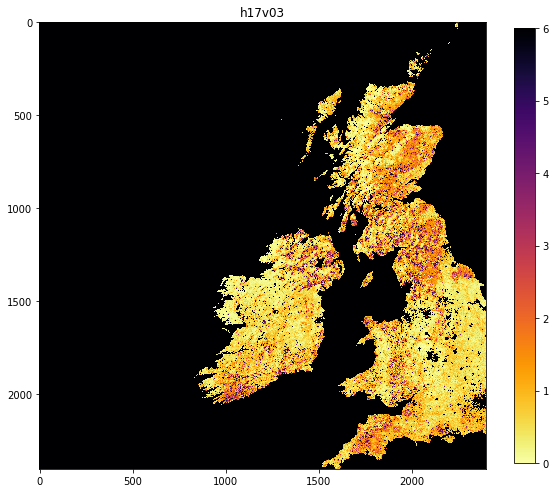
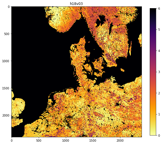
3.3.3.2 reading and displaying image data
Let’s now read some data as above.
we do this with:
g.Open(gdal_fname)
data = g.ReadAsArray()
Originally the data are uint8 (unsigned 8 bit data), but we need to
multiply them by scale_factor (0.1 here) to convert to physical
units. This also casts the data type to float.
We can straightforwardly plot the images using matplotlib. We first
importt the library:
import matplotlib.pylab as plt
Then set up the figure size:
plt.figure(figsize=(10,10))
Plot the image:
plt.imshow( data, vmin=0, vmax=6,cmap=plt.cm.inferno_r)
where here data is a 2-D dataset. We can set limits to the image
scaling (vmin, vmax), so that we emphasise a particular range of
values, and we can apply custom colourmaps (cmap=plt.cm.inferno_r).
Finally here, we set a title, and plot a colour wedge to show the data
scale. The scale=0.8 here allows us to align the size of the scale
with the plotted image size.
plt.title(dataset_name)
plt.colorbar(shrink=0.8)
If we want to save the plotted image to a file, e.g. in the directory
images, we use:
plt.savefig(out_filename)
import gdal
from pathlib import Path
import matplotlib.pylab as plt

# get only v03 hdf names
filenames = sorted(Path('data').glob('*2018*v03*.hdf'))


out_directory = Path('images')

for filename in filenames:
    # pull the tile name from the filename
    # to use as plot title
    tile = filename.name.split('.')[2]

    dataset_name = f'HDF4_EOS:EOS_GRID:"{str(filename):s}\":MOD_Grid_MCD15A3H:Lai_500m'
    g = gdal.Open(dataset_name)
    data = g.ReadAsArray()
    scale_factor = float(g.GetMetadata()['scale_factor'])

    print(dataset_name,scale_factor)
    print('*'*len(dataset_name))
    print(type(data),data.dtype,data.shape,'\n')

    data = data * scale_factor
    print(type(data),data.dtype,data.shape,'\n')
    plt.figure(figsize=(10,10))
    plt.imshow( data, vmin=0, vmax=6,cmap=plt.cm.inferno_r)
    plt.title(tile)
    plt.colorbar(shrink=0.8)

    # save figure as png
    plot_name = filename.stem + '.png'
    print(plot_name)
    out_filename = out_directory.joinpath(plot_name)
    plt.savefig(out_filename)
HDF4_EOS:EOS_GRID:"data/MCD15A3H.A2018273.h17v03.006.2018278143630.hdf":MOD_Grid_MCD15A3H:Lai_500m 0.1
**********************************************************************************************
<class 'numpy.ndarray'> uint8 (2400, 2400)

<class 'numpy.ndarray'> float64 (2400, 2400)

MCD15A3H.A2018273.h17v03.006.2018278143630.png
HDF4_EOS:EOS_GRID:"data/MCD15A3H.A2018273.h18v03.006.2018278143633.hdf":MOD_Grid_MCD15A3H:Lai_500m 0.1
**********************************************************************************************
<class 'numpy.ndarray'> uint8 (2400, 2400)

<class 'numpy.ndarray'> float64 (2400, 2400)

MCD15A3H.A2018273.h18v03.006.2018278143633.png
# Let's check the images we saved are there!
# and access some file info while we are here
# using pathlib
from pathlib import Path
from datetime import datetime

for f in Path('images').glob('MCD*2018*v03*.png'):

    # get the file size in bytes
    size_in_B = f.stat().st_size

    # get the file modification time (ns)
    mod_date_ns = f.stat().st_mtime_ns
    mod_date = datetime.fromtimestamp(mod_date_ns // 1000000000)

    print(f'{f} {size_in_B} Bytes {mod_date}')
images/MCD15A3H.A2018273.h18v03.006.2018278143633.png 297318 Bytes 2018-10-19 16:59:20
images/MCD15A3H.A2018273.h17v03.006.2018278143630.png 142654 Bytes 2018-10-19 16:59:19
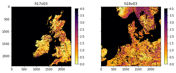
3.3.3.3 subplot plotting
Often, we want to have several figures on the same plot. We can do this
with plt.subplots():
The way we set the title and other features is slightly diifferent, but there are many example of different plot types on the web we can follow as examples.
import gdal
from pathlib import Path
import matplotlib.pylab as plt
import numpy as np

filenames = sorted(Path('data').glob('*2018*v03*.hdf'))

out_directory = Path('images')

'''
Set up subplots of 1 row x 2 columns
'''
fig, axs = plt.subplots(nrows=1, ncols=2, sharex=True, sharey=True,
                       figsize=(10,5))
# need to force axs collapse to a 2D array
# for indexing to be easy T here is transpose
# to get row/col the right way around
axs = np.array(axs).T.flatten()

for i,filename in enumerate(filenames):
    # pull the tile name from the filename
    # to use as plot title
    tile = filename.name.split('.')[2]


    dataset_name = f'HDF4_EOS:EOS_GRID:"{str(filename):s}\":MOD_Grid_MCD15A3H:Lai_500m'
    g = gdal.Open(dataset_name)
    data = g.ReadAsArray() * float(g.GetMetadata()['scale_factor'])

    img = axs[i].imshow(data, interpolation="nearest", vmin=0, vmax=4,
                 cmap=plt.cm.inferno_r)
    axs[i].set_title(tile)
    plt.colorbar(img,ax=axs[i],shrink=0.7)

# save figure as pdf this time
plot_name = 'joinedup.pdf'
print(plot_name)
out_filename = out_directory.joinpath(plot_name)
plt.savefig(out_filename)
joinedup.pdf
Exercise 3.3.5
We now want to use the additional files:
MCD15A3H.A2018273.h17v04.006.2018278143630.hdf
MCD15A3H.A2018273.h18v04.006.2018278143638.hdf
- copy and change the code above to use files of the pattern
*v0[3,4]*.hdf - use subplot as above to plot a 2x2 set of subplots of these data.
Hint
The code should look much like that above, but you need to give the fiuller list of filenames and set the subplot shape.
The code [3,4] in the pattern *v0[3,4]*.hdf means match either
3 or 4, so the pattern must be *v03*.hdf or *v03*.hdf.
The result should look like:
# do exercise here
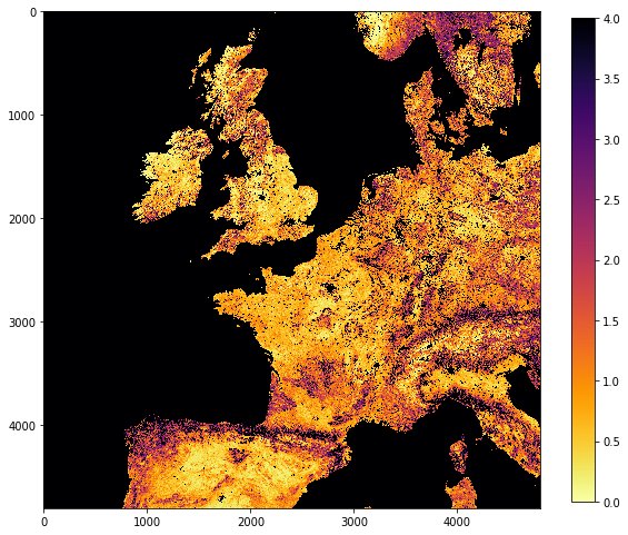
3.3.3.3 tile stitching
You may want to generate a single view of the 4 tiles.
We could achieve this by stitching things together “by hand”…
recipe:
First, lets generate a 3D dataset with all 4 tiles, so we have the images stored as members of a list
data[0],data[1],data[2]anddata[3]:data = [] for filename in filenames: dataname = f'HDF4_EOS:EOS_GRID:"{str(filename):s}":MOD_Grid_MCD15A3H:Lai_500m' g = gdal.Open(dataname) data.append(g.ReadAsArray() * scale)
then, we produce vertical stacks of the first two and last two files. This can be done in various ways, but it is perhaps clearest to use
np.vstack()top = np.vstack([data[0],data[1]]) bot = np.vstack([data[2],data[3]])
then, produce a horizontal stack of these stacks:
lai_stich = np.hstack([top,bot])
and plot the dataset
import gdal
from pathlib import Path
import matplotlib.pylab as plt
scale = 0.1
filenames = sorted(Path('data').glob('*2018*v0*.hdf'))
data = []
for filename in filenames:
dataname = f'HDF4_EOS:EOS_GRID:"{str(filename)}":MOD_Grid_MCD15A3H:Lai_500m'
g = gdal.Open(dataname)
# append each image to the data list
data.append(g.ReadAsArray() * scale)
top = np.vstack([data[0],data[1]])
bot = np.vstack([data[2],data[3]])
lai_stich = np.hstack([top,bot])
plt.figure(figsize=(10,10))
plt.imshow(lai_stich, interpolation="nearest", vmin=0, vmax=4,
cmap=plt.cm.inferno_r)
plt.colorbar(shrink=0.8)
<matplotlib.colorbar.Colorbar at 0x126b0fac8>
Exercise 3.3.6
- examine how the
vstackandhstackmethods work. Print out the shape of the array after stacking to appreciate this. - how big (in pixels) is the whole dataset now?
- If a
floatis 64 bits, how many bytes is this data array likely to be?
# do exercise here
3.3.3.4 gdal virtual file
However, stitching in this way is problematic if you want to mosaic many tiles, as you need to read in all the data in memory. Also,some tiles may be missing. GDAL allows you to create a mosaic as virtual file format, using gdal.BuildVRT (check the documentation).
This function takes two inputs: the output filename (stitch_up.vrt)
and a set of GDAL format filenames. It returns the open output dataset,
so that we can check what it looks like with e.g. gdal.Info
import gdal
from pathlib import Path

# need to convert filenames to strings
# which we can do with p.as_posix() or str(p)
filenames = sorted([p.as_posix() for p in Path('data').glob('*273*v0[3,4]*.hdf')])
datanames = [f'HDF4_EOS:EOS_GRID:"{str(filename)}":MOD_Grid_MCD15A3H:Lai_500m' \
                for filename in filenames]
stitch_vrt = gdal.BuildVRT("stitch_up.vrt", datanames)

print(gdal.Info(stitch_vrt))
Driver: VRT/Virtual Raster
Files: stitch_up.vrt
Size is 4800, 4800
Coordinate System is:
PROJCS["unnamed",
    GEOGCS["Unknown datum based upon the custom spheroid",
        DATUM["Not specified (based on custom spheroid)",
            SPHEROID["Custom spheroid",6371007.181,0]],
        PRIMEM["Greenwich",0],
        UNIT["degree",0.0174532925199433]],
    PROJECTION["Sinusoidal"],
    PARAMETER["longitude_of_center",0],
    PARAMETER["false_easting",0],
    PARAMETER["false_northing",0],
    UNIT["Meter",1]]
Origin = (-1111950.519667000044137,6671703.117999999783933)
Pixel Size = (463.312716527916677,-463.312716527708290)
Corner Coordinates:
Upper Left  (-1111950.520, 6671703.118) ( 20d 0' 0.00"W, 60d 0' 0.00"N)
Lower Left  (-1111950.520, 4447802.079) ( 13d 3'14.66"W, 40d 0' 0.00"N)
Upper Right ( 1111950.520, 6671703.118) ( 20d 0' 0.00"E, 60d 0' 0.00"N)
Lower Right ( 1111950.520, 4447802.079) ( 13d 3'14.66"E, 40d 0' 0.00"N)
Center      (       0.000, 5559752.598) (  0d 0' 0.01"E, 50d 0' 0.00"N)
Band 1 Block=128x128 Type=Byte, ColorInterp=Gray
  NoData Value=255
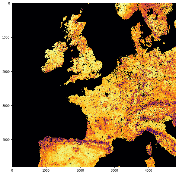
So we see that we now have 4800 columns by 4800 rows dataset, centered around 0 degrees North, 0 degrees W. Let’s plot the data…
# stitch_vrt is an already opened GDAL dataset, needs to be read in
plt.figure(figsize=(10,10))
plt.imshow(stitch_vrt.ReadAsArray()*0.1,
           interpolation="nearest", vmin=0, vmax=6,
          cmap=plt.cm.inferno_r)
<matplotlib.image.AxesImage at 0x10a0ecda0>
3.3.4 The country borders dataset
A number of vectors with countries and administrative subdivisions are
available. The TM_WORLD_BORDERS
shapefile
is popular and in the public domain. You can see it, and have a look at
the data
here. We
need to download and unzip this file… We’ll use requests as before, and
we’ll unpack the zip file using
`shutil.unpack_archive <https://docs.python.org/3/library/shutil.html#shutil.unpack_archive>`__
import requests
import shutil

tm_borders_url = "http://thematicmapping.org/downloads/TM_WORLD_BORDERS-0.3.zip"

r = requests.get(tm_borders_url)
with open("data/TM_WORLD_BORDERS-0.3.zip", 'wb') as fp:
    fp.write (r.content)

shutil.unpack_archive("data/TM_WORLD_BORDERS-0.3.zip",
                     extract_dir="data/")
Make sure you have the relevant files available in your data folder!
We can then inspect the dataset using the command line tool ogrinfo.
We can call it from the shell by appending the ! symbol, and select
that we want to check only the data for the UK (stored in the FIPS
field with value UK):
It is worth noting that using OGR’s queries trying to match a string,
the string needs to be surrounded by '. You can also use more
complicated SQL queries if you wanted to.
!ogrinfo -nomd -geom=NO -where "FIPS='UK'" data/TM_WORLD_BORDERS-0.3.shp TM_WORLD_BORDERS-0.3
INFO: Open of `data/TM_WORLD_BORDERS-0.3.shp'
      using driver `ESRI Shapefile' successful.

Layer name: TM_WORLD_BORDERS-0.3
Geometry: Polygon
Feature Count: 1
Extent: (-180.000000, -90.000000) - (180.000000, 83.623596)
Layer SRS WKT:
GEOGCS["GCS_WGS_1984",
    DATUM["WGS_1984",
        SPHEROID["WGS_84",6378137.0,298.257223563]],
    PRIMEM["Greenwich",0.0],
    UNIT["Degree",0.0174532925199433],
    AUTHORITY["EPSG","4326"]]
FIPS: String (2.0)
ISO2: String (2.0)
ISO3: String (3.0)
UN: Integer (3.0)
NAME: String (50.0)
AREA: Integer (7.0)
POP2005: Integer64 (10.0)
REGION: Integer (3.0)
SUBREGION: Integer (3.0)
LON: Real (8.3)
LAT: Real (7.3)
OGRFeature(TM_WORLD_BORDERS-0.3):206
  FIPS (String) = UK
  ISO2 (String) = GB
  ISO3 (String) = GBR
  UN (Integer) = 826
  NAME (String) = United Kingdom
  AREA (Integer) = 24193
  POP2005 (Integer64) = 60244834
  REGION (Integer) = 150
  SUBREGION (Integer) = 154
  LON (Real) = -1.600
  LAT (Real) = 53.000
We inmediately see that the coordinates for the UK are in several polygons, and in WGS84 (Latitude and Longitude in decimal degrees). This is incompatible with the MODIS data (SIN projection), but fortunately GDAL understands about coordinate systems.
We can use GDAL to quickly apply the vector feature for the UK as a mask. There are several ways of doing this, but the simplest is to use gdal.Warp (the link is to the command line tool). In this case, we just want to create:
- an in-memory (i.e. not saved to a file) dataset. We can use the
format
MEM, so no file is written out. - where the
FIPSfield is equal to'UK', we want the LAI to show, elsewhere, we set it to some value to indicate “no data” (e.g. -999)
The mosaicked version of the MODIS LAI product is in called
stitch_up.vrt. Since we’re not saving the output to a file (MEM
output option), we can leave the output as an empty string "". The
shapefile comes with the cutline options:
cutlineDSNamethat’s the name of the vector file we want to use as a cutlinecutlineWherethat’s the selection statement for the attribute table in the dataset.
To set the no data value to 200, we can use the option
dstNodata=200. This is because very large values in the LAI product
are already indicated to be invalid.
We can then just very quickly perform this and check…
import gdal
import matplotlib.pylab as plt
from pathlib import Path

filenames = sorted([p.as_posix() for p in Path('data').glob('*2018*v0*.hdf')])
datanames = [f'HDF4_EOS:EOS_GRID:"{str(filename)}":MOD_Grid_MCD15A3H:Lai_500m' \
                for filename in filenames]
stitch_vrt = gdal.BuildVRT("stitch_up.vrt", datanames)


g = gdal.Warp("", "stitch_up.vrt",
         format = 'MEM',dstNodata=200,
          cutlineDSName = 'data/TM_WORLD_BORDERS-0.3.shp', cutlineWhere = "FIPS='UK'")

# read and plot data
masked_lai = g.ReadAsArray()*0.1
plt.figure(figsize=(10,10))
plt.title('Red white and blue: Brexit UK')
plt.imshow(masked_lai, interpolation="nearest", vmin=1, vmax=3,
          cmap=plt.cm.RdBu)
<matplotlib.image.AxesImage at 0x126942320>
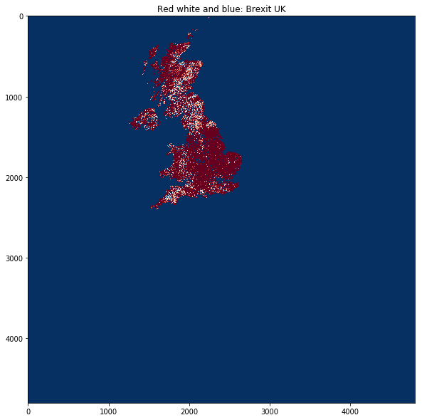
So that works as expected, but since we haven’t actually told GDAL anything about the output (other than apply the mask), we still have a 4800 pixel wide dataset.
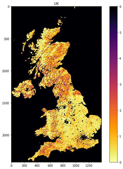
You may want to crop it by looking for where the original dataset is valid (0 to 100 here). This will generally save a lot of computer memory. You’ll be pleased to know that this is a great slicing application!
import numpy as np

lai = g.ReadAsArray()

# data valid where lai <= 100 here
valid_mask = np.where(lai <= 100)

# work out the bounds of valid_mask
min_y      = valid_mask[0].min()
max_y      = valid_mask[0].max() + 1

min_x      = valid_mask[1].min()
max_x      = valid_mask[1].max() + 1

# now slice, and scale LAI
lai = lai[min_y:max_y,
          min_x:max_x]*0.1

plt.figure(figsize=(10,10))
plt.imshow(lai, vmin=0, vmax=6,
           cmap=plt.cm.inferno_r)
plt.title('UK')
plt.colorbar()
<matplotlib.colorbar.Colorbar at 0x12a6486d8>
Exercise 3.3.7 Homework
- Develop a function that takes the list of dataset names and the
information you passed to
gdal.Warp(or a subset of this) and returns a cropped image of valid data. - Use this function to show separate images of: France, Belgium, the Netherlands
# do exercise here
Exercise 3.3.8 Homework
- Download data for these same four tiles from the MODIS snow cover dataset for some particular date (in winter). Check the related quicklooks to see that the dataset isn’t all covered in cloud.
- show the snow cover for one or more selected countries.
- calculate summary statistics for the datasets.
Hint the codes would be very similar to above, but watch out for the scaling factor not being the same (no scaling for the snow cover!). Also, watch out for the dataset being on a different NASA server to the LAI data (as in exercise above).
When you calculate summary statistics, make sure you ignore all invalid
pixels. You could do that by generating a mask of the dataset (after you
have clipped it) using np.where(), and only process those pixels,
e.g.:
image[np.where(image<=100)].mean()
rather than
image.mean()
as the latter would include invalid pixels.
# do exercise here