3.6 Reconciling projections
Table of Contents
3.6 Reconciling projections
3.6.1 Introduction
3.6.1.1 Projections
3.6.1.2 Changing Projections
3.6.2 Requirements
3.6.2.1 Run the pre-requisite scripts
3.6.3 Reconcile the datasets
3.6.3.1 load an exemplar dataset
3.6.3.2 get information from source file
3.6.3.4 reprojection
3.6.3.5 crop
3.6.3.6 Putting this together
3.6.6 Summary
3.6.1 Introduction
This section of notes is optional to the course, and the tutor may decide not to go through this in class.
That said, the information and examples contained here can be very useful for accessing and processing certain types of geospatial data.
In particular, we deal with obtaining climate data records from
ECMWF
that we will later use for model fitting. These data come in a
netcdf
format (commonly used for climate data) with a grid in
latitude/longitude. To ‘overlay’ these data with another dataset
(e.g. the MODIS LAI product that we have been using) in a different
(equal area) projection, we use the gdal function
gdal.ReprojectImage(src, dst, src_proj, dst_proj, interp)
where:
src      : a source dataset that we want to process
dst      : a blank destination dataset that we set up with the
           required (output) data type, shape, and geotransform and projection
src_proj : the source dataset projection wkt
dst_proj : the destination projection wkt
interp   : the required interpolation method, e.g. gdalconst.GRA_Bilinear
where wkt stands for well known text and is a projection format string.
Other codes we use are ones we have developed earlier.
In these notes, we will learn:
* how to access an ECMWF daily climate dataset (from ERA interim)
* how to reproject the dataset to match another spatial dataset (MODIS LAI)
We will then save some datasets that we will use later in the notes. For this reason, it’s possile to skip this section, and return to it later.
3.6.1.1 Projections
For various reasons, different geospatial datasets will come in different projections.
Considering for example, satellite-derived data from Low Earth Orbit LEO, the satellite sensor will typically obtain image data in a swath as it passes over the Earth surface. Projected onto the Earth surface, this appears as a strip of data:
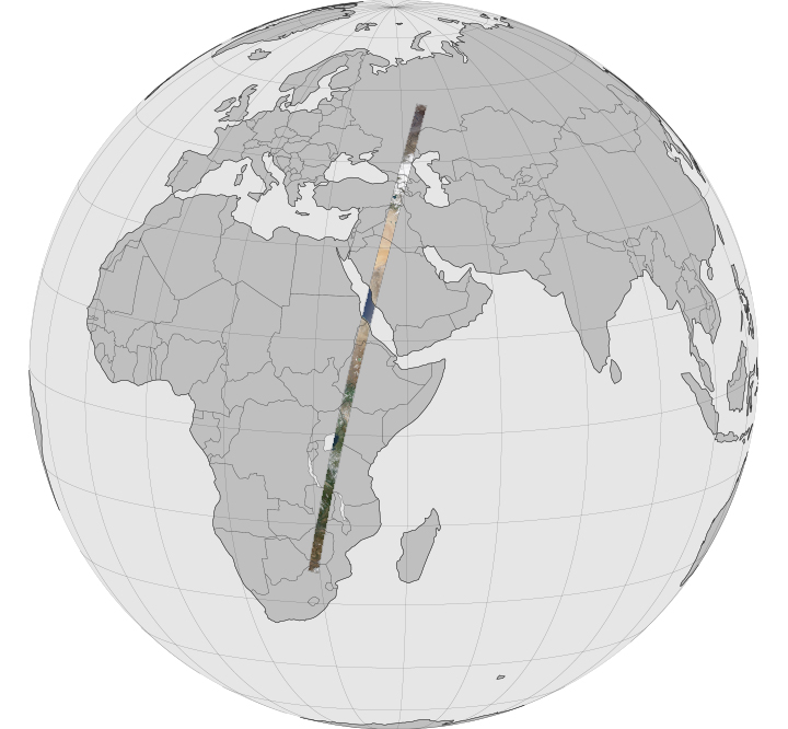
but in the satellite data recording system, the data are stored as a regular array. We call such satellite data ‘swath’ (or ‘swath-like’) data (in the satellite imager coordinate system) and we may obtain data products in anything up to Level 2 in such a form.
These data are often difficult for data scientists to deal with. They generally prefer to have a dataset mapped to a uniform space-time grid, even though this may involve some re-sampling, which can sometimes result in loss of information. The convenience of a uniform space-time grid means that you can. for example, look at dynamic features (information over time).
The properties of the ‘uniform space-time grid’ will depend on user requirements. For some, it is important to have an equal area projection, one where the ‘pixel size’ is consistent throughout the dataset.
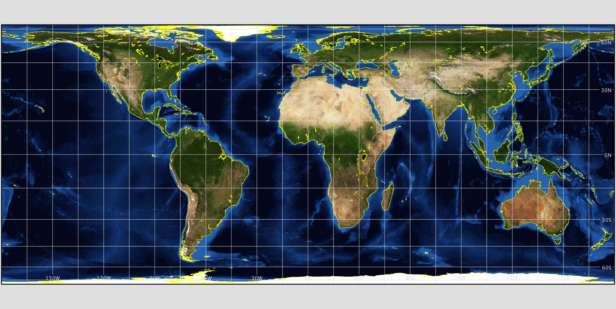
even if this is not convenient for viewing some areas of the Earth (map projections are very political!).
Or other factors may be more important, such as user familiarity with a simple latitude/longitude grid typically used by climate scientists.
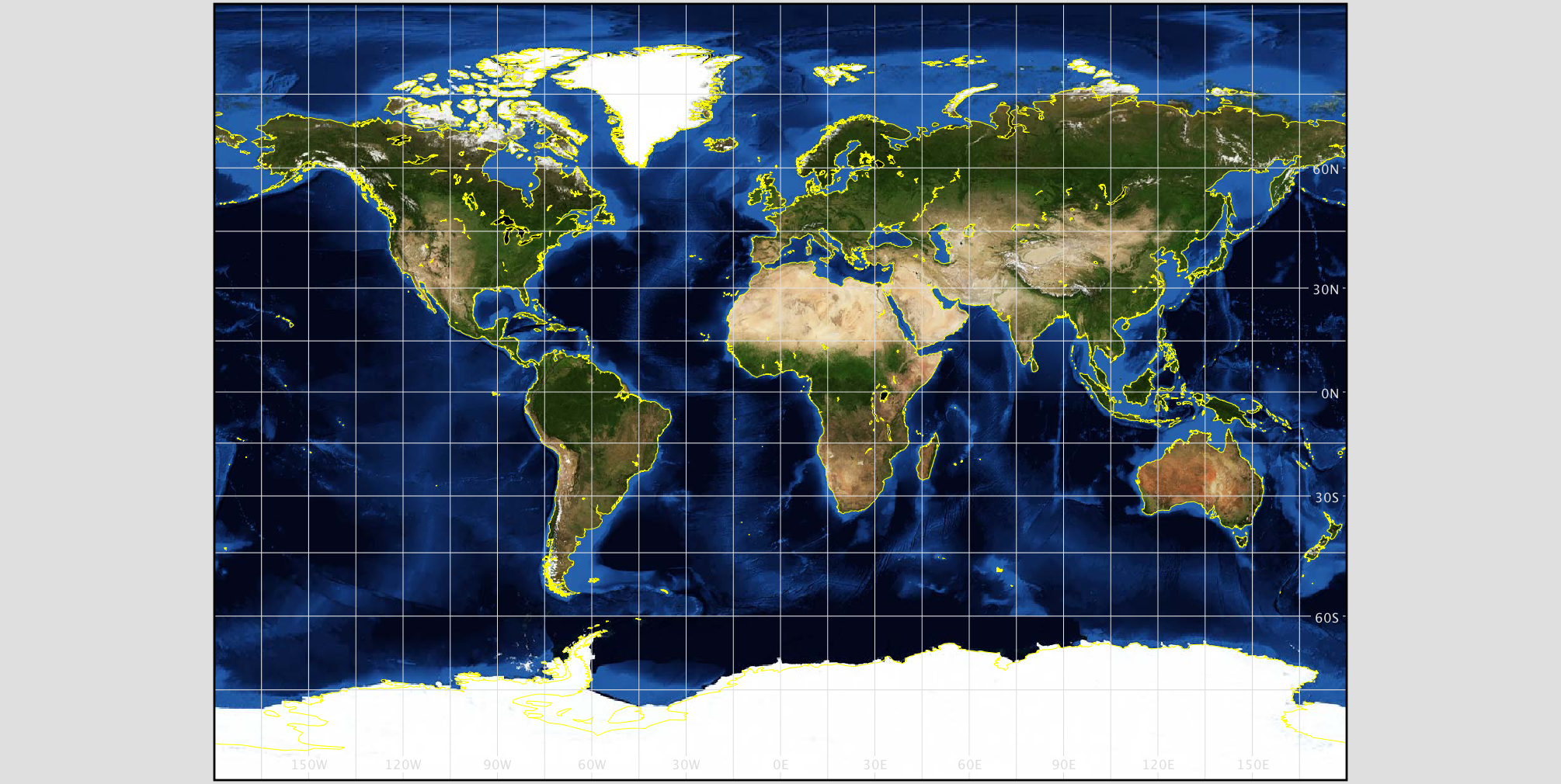
For others, a conformal projection (preserving angles, as a cost of distance distortion) may be vital.
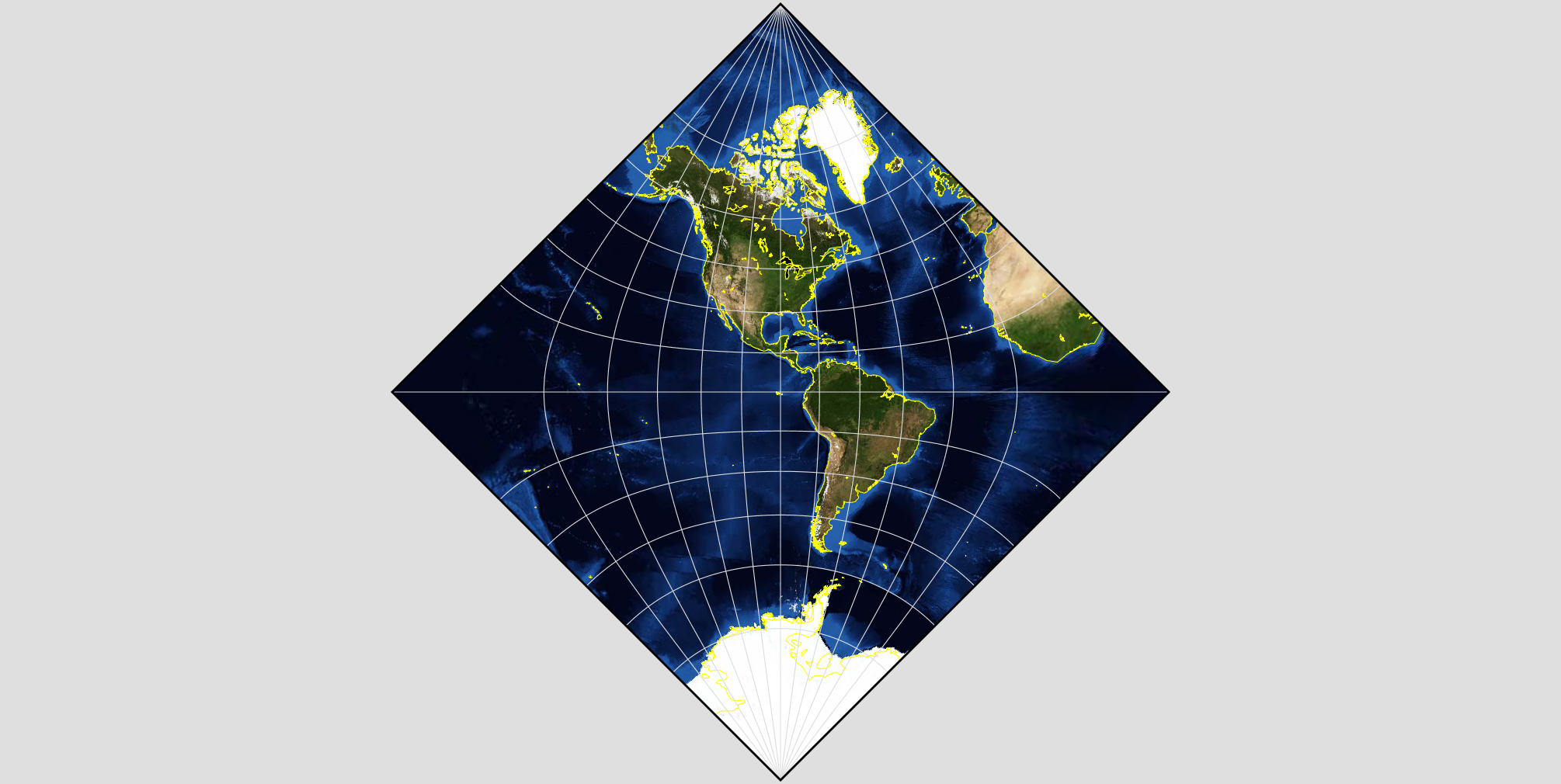
We have see that MODIS data products, for example, come described in an equal area sinusoidal grid:
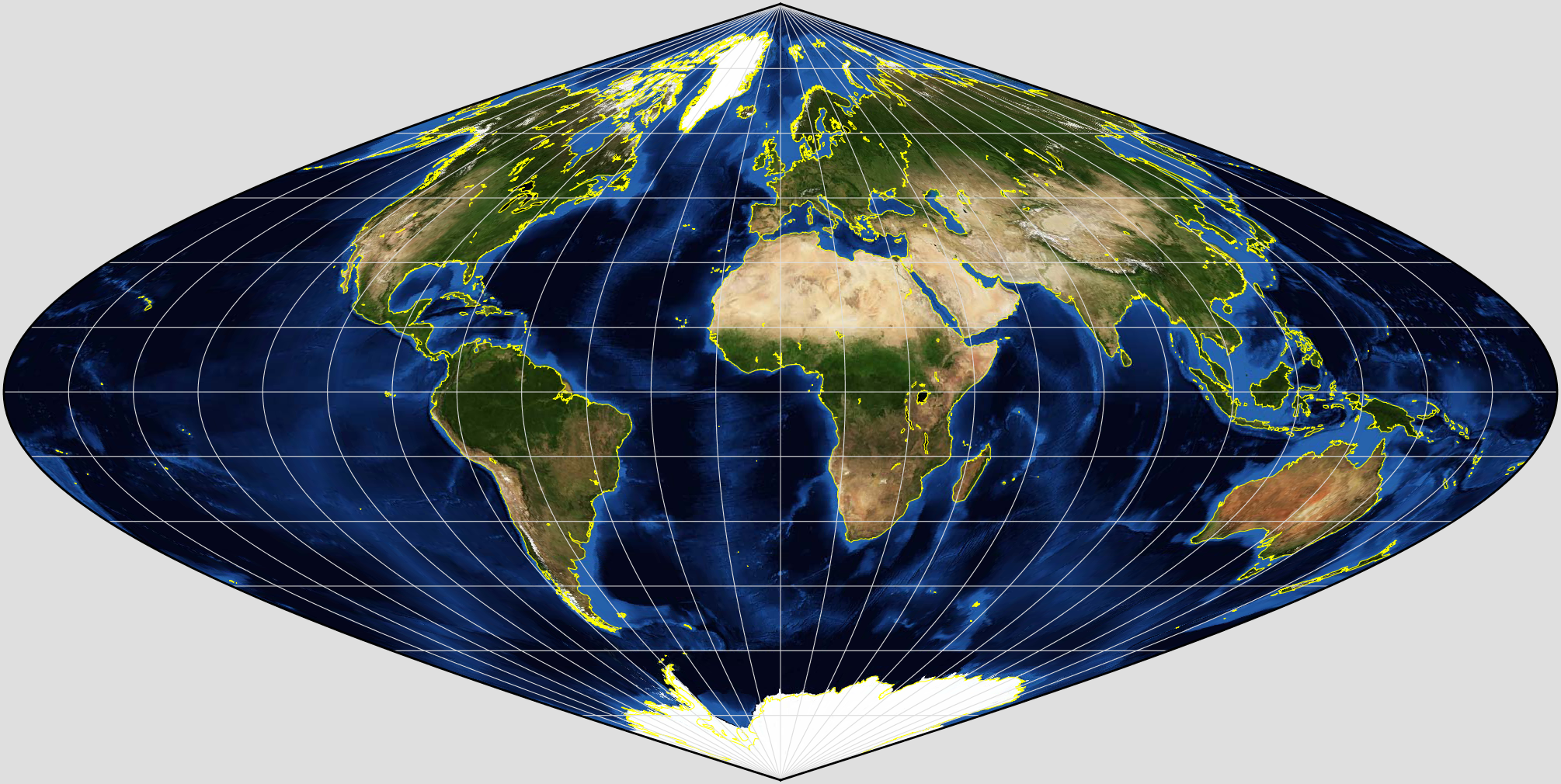 .
.
but the data for high latitudes and longitudes appears very distorted.
We must accept then, that dealing with geospatial data must involve some understanding of projections, as well as practically, how to convert datasets between different projections.
Earth shape
One factor that can make life even more complicated than using just different projections is the use of different assumptions about the Earth shape (e.g. sphere, spheroid, radius variations). Often, the particular assumptions used by a group of users is just a result of history: it is what has ‘traditionally’ used for that purpose. It can be seen as too bothersome or expensive to change this.
Since we can convert between different projections though, we can also deal with different Earth shape assumptions. We just have to be very clear about what was assumed. If at all possible, the geospatial datasets themselves should contain a full description of the projection and Earth shape assumed, but this is not always the case.
The datasets we will mostly be dealing are in the following projections:
MODIS Sinusoidal (tested), which assumes a custom spherical Earth of radius 6371007.181 m. In
cartopythis is given as Sinusoidal.MODIS:# MODIS data products use a Sinusoidal projection of a spherical Earth # http://modis-land.gsfc.nasa.gov/GCTP.html Sinusoidal.MODIS = Sinusoidal(globe=Globe(ellipse=None, semimajor_axis=6371007.181, semiminor_axis=6371007.181))
In the MODIS data hdf products, the projection information is stored directly. Extracted as a wkt, this is:
[[PROJCS["unnamed",
    GEOGCS["Unknown datum based upon the custom spheroid",
        DATUM["Not_specified_based_on_custom_spheroid",
            SPHEROID["Custom spheroid",6371007.181,0]],
    PRIMEM["Greenwich",0],
    UNIT["degree",0.0174532925199433]],
PROJECTION["Sinusoidal"],
PARAMETER["longitude_of_center",0],
PARAMETER["false_easting",0],
PARAMETER["false_northing",0],
UNIT["metre",1,AUTHORITY["EPSG","9001"]]]
According to SR-ORG, the MODIS projection uses a spherical projection ellipsoid but a WGS84 datum ellipsoid. This is not quite the same as the definition in the wkt above.
It is also defined by SR-ORG with the EPSG code 6974 for software that can use
semi_majorandsemi_minorprojection definitions.Some software may use the simpler 6965 definition (or the older 6842).
The MODIS projection 6974 is given as:
PROJCS["MODIS Sinusoidal",
    GEOGCS["WGS 84",
        DATUM["WGS_1984",
            SPHEROID["WGS 84",6378137,298.257223563,
                AUTHORITY["EPSG","7030"]],
        AUTHORITY["EPSG","6326"]],
    PRIMEM["Greenwich",0,
        AUTHORITY["EPSG","8901"]],
    UNIT["degree",0.01745329251994328,
        AUTHORITY["EPSG","9122"]],
    AUTHORITY["EPSG","4326"]],
PROJECTION["Sinusoidal"],
PARAMETER["false_easting",0.0],
PARAMETER["false_northing",0.0],
PARAMETER["central_meridian",0.0],
PARAMETER["semi_major",6371007.181],
PARAMETER["semi_minor",6371007.181],
UNIT["m",1.0],
AUTHORITY["SR-ORG","6974"]]
None of these codes are defined in
gdal(see files in $GDAL_DATA/*.wkt for details), so to use them, we have to take the file from SR-ORG.For the datasets we are using, it makes no real difference whether the projection information from the file is used instead of MODIS projection 6974, so we will use that from the file. For other areas and especially for any higher spatial resolution datasets, it is worth investigating which is more appropriate.
ECMWF netcdf format (derived from GRIB) ERA Interim climate datasets (1979-Present). These are geographic coordinates (latitude/longitude) in a custom spheroid with a radius 6371200 m.
This information can be obtained from any example of a GRIB file, as we shall see below. As a wkt, this is:
['GEOGCS["Coordinate System imported from GRIB file",
DATUM["unknown",SPHEROID["Sphere",6371200,0]],
PRIMEM["Greenwich",0],UNIT["degree",0.0174532925199433]]']
A more common spheroid to use is WGS84, although even in that case there are multiple ‘realisations’ available (used mainly by the DoD). Users should generally implement that given in EPSG code 4326 used by the GPS system, for example.
[GEOGCS["WGS 84",
    DATUM["WGS_1984",
        SPHEROID["WGS 84",6378137,298.257223563,
            AUTHORITY["EPSG","7030"]],
        AUTHORITY["EPSG","6326"]],
    PRIMEM["Greenwich",0,
        AUTHORITY["EPSG","8901"]],
    UNIT["degree",0.01745329251994328,
        AUTHORITY["EPSG","9122"]],
    AUTHORITY["EPSG","4326"]]]
3.6.1.2 Changing Projections
We can conveniently use the Python
`cartopy <https://scitools.org.uk/cartopy/docs/v0.16/>`__ package to
explore projections.
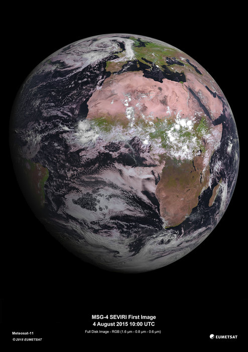
We download an image taken from the satellite sensor (SEVIRI):

The sensor builds up images of the Earth disc from geostationarty orbit, actioned by the platform spin.
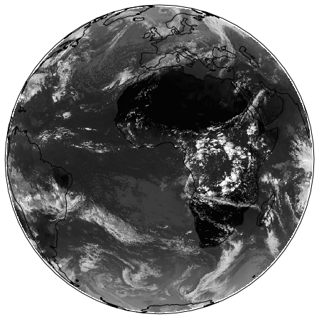
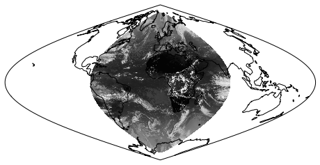
In the code below, we plot the dataset in the ‘earth disk’ (Orthographic) projection, then re-map it to the equal area Sinusoidal projection.
try:
    from urllib2 import urlopen
except ImportError:
    from urllib.request import urlopen
from io import BytesIO
%matplotlib inline

import cartopy.crs as ccrs
import matplotlib.pyplot as plt
are_you_sure = False

'''
=====================================================
Don't run this cell in class as it will take too long!

                 Use it for homework
                 set are_you_sure = True
=====================================================
'''

'''
from https://scitools.org.uk/cartopy/docs/v0.16/\
            gallery/geostationary.html#sphx-glr-gallery-geostationary-py
'''
def geos_image():
    """
    Return a specific SEVIRI image by retrieving it from a github gist URL.

    Returns
    -------
    img : numpy array
        The pixels of the image in a numpy array.
    img_proj : cartopy CRS
        The rectangular coordinate system of the image.
    img_extent : tuple of floats
        The extent of the image ``(x0, y0, x1, y1)`` referenced in
        the ``img_proj`` coordinate system.
    origin : str
        The origin of the image to be passed through to matplotlib's imshow.

    """
    url = ('https://gist.github.com/pelson/5871263/raw/'
           'EIDA50_201211061300_clip2.png')
    img_handle = BytesIO(urlopen(url).read())
    img = plt.imread(img_handle)
    img_proj = ccrs.Geostationary(satellite_height=35786000)
    img_extent = [-5500000, 5500000, -5500000, 5500000]
    return img, img_proj, img_extent, 'upper'

if are_you_sure:
    print('Retrieving image...')
    img, crs, extent, origin = geos_image()

    fig = plt.figure(figsize=(8,8))
    ax = fig.add_subplot(1, 1, 1,projection=\
                         ccrs.Orthographic(central_longitude=0.0, central_latitude=0.0))
    ax.coastlines()
    ax.set_global()
    ax.imshow(img, transform=crs, extent=extent, origin=origin, cmap='gray')

    fig = plt.figure(figsize=(8,8))
    ax = fig.add_subplot(1, 1, 1, projection=\
                         ccrs.Sinusoidal(central_longitude=0.0, \
                            false_easting=0.0, false_northing=0.0))
    ax.coastlines()
    ax.set_global()
    print('Projecting and plotting image (this may take a while)...')
    ax.imshow(img, transform=crs, extent=extent, origin=origin, cmap='gray')
Retrieving image...
Projecting and plotting image (this may take a while)...
The full list of `cartopy
projections <https://scitools.org.uk/cartopy/docs/v0.16/crs/projections.html>`__
is quite entensive.
Exercise 3.6.1 Extra Homework
- Explore some different types of projection using
cartopyand make a note of their features. - Read up (follow the links in the text above) on projections.
#do exercise here
3.6.2 Requirements
We will need to:
- make sure we have the MODIS LAI dataset locally
- read them in for a given country.
- register with ecmwf, install ecmwfapi
- get the temperature datasset from ECMWF for 2006 and 2017 for Europe
- get the country borders shapefile
Set up the conditions
# required general imports
import matplotlib.pyplot as plt
%matplotlib inline
import numpy as np
import sys
import os
from pathlib import Path
import gdal
from datetime import datetime, timedelta
import cartopy.crs as ccrs
'''
Set the country code and year to be used here
'''
country_code = 'UK'
year = 2017
shpfile = "data/TM_WORLD_BORDERS-0.3.shp"
3.6.2.1 Run the pre-requisite scripts
Make sure you register with ECMWF * register with ECMWF and install the API
Follow the [ECMWF instructions](https://confluence.ecmwf.int/display/WEBAPI/Access+ECMWF+Public+Datasets)
Sort data prerequisities * Run the codes in the prerequisites section
OR
- Run the [prerequisites script]:
# install ecmwf api -- do this once only
ECMWF = 'https://software.ecmwf.int/wiki/download/attachments/56664858/ecmwf-api-client-python.tgz'
try:
    from ecmwfapi import ECMWFDataServer
except:
    try:
        !pip install $ECMWF
    except:
        # on Unix/Linux
        !pip install --user $ECMWF
# just make sure the pre-requisites are run
%run geog0111/Chapter3_6A_prerequisites.py $country_code $year
['geog0111/Chapter3_6A_prerequisites.py', 'UK', '2017'] 2017 UK
Looking for match to sample  2017-01-01 00:00:00
Looking for match to sample  2017-02-10 00:00:00
Looking for match to sample  2017-03-22 00:00:00
Looking for match to sample  2017-05-01 00:00:00
Looking for match to sample  2017-06-10 00:00:00
Looking for match to sample  2017-07-20 00:00:00
Looking for match to sample  2017-08-29 00:00:00
Looking for match to sample  2017-10-08 00:00:00
Looking for match to sample  2017-11-17 00:00:00
Looking for match to sample  2017-12-27 00:00:00
18.45137418797783
0.19862203366558234
(2624, 1396, 92) (2624, 1396, 92)
interpolating ...
(2624, 1396, 92)
saving ...
europe_data_2016_2017.nc exists
GEOGCS["Coordinate System imported from GRIB file",DATUM["unknown",SPHEROID["Sphere",6371200,0]],PRIMEM["Greenwich",0],UNIT["degree",0.0174532925199433]]
Refreshing nc file europe_data_2016_2017.nc
data/europe_data_2016.nc
data/europe_data_2017.nc
# read in the LAI data for given country code
tiles = []
for h in [17, 18]:
    for v in [3, 4]:
        tiles.append(f"h{h:02d}v{v:02d}")

fname = f'lai_data_{year}_{country_code}.npz'
ofile = Path('data')/fname
try:
    # read data from npz file
    lai = np.load(ofile)
    print(lai['lai'].shape)
except:
    print(f"{ofile} doesn't exist: sort the pre-requisites")
(2624, 1396, 92)
import numpy as np
# a quick look at some stats to see if there are data there
# and they are sensible
lai = np.load(ofile)
print(np.array(lai['lai'][1000,700]),\
      np.array(lai['weights'][1000,700]))
# does it have the interpolated value?
if 'interpolated_lai' in list(lai.keys()):
    print(np.array(lai['interpolated_lai'][1000,700]))
[1.1 1.1 1.2 0.9 0.9 1.2 1.  0.8 1.4 0.3 0.  0.5 0.3 0.9 0.6 1.  0.7 0.5
 0.7 0.6 1.3 0.7 0.1 1.  1.  0.6 1.1 0.5 1.1 1.  1.1 1.1 1.1 0.  0.6 1.4
 1.3 1.6 1.7 1.7 1.1 0.3 1.3 1.7 1.5 1.2 0.5 0.6 1.6 3.1 0.3 2.  1.6 0.5
 2.6 2.5 0.4 0.4 0.4 0.4 0.4 1.1 1.7 0.5 1.5 1.4 0.1 1.4 1.  1.  0.3 1.1
 0.2 1.1 0.1 0.7 2.6 1.7 2.  1.4 1.4 0.3 0.4 0.7 1.1 1.1 0.8 0.8 0.9 1.2
 1.2 1.2] [0.38196601 0.38196601 0.38196601 0.38196601 0.38196601 0.38196601
 0.38196601 0.38196601 0.38196601 0.38196601 0.38196601 1.
 1.         1.         1.         1.         1.         1.
 1.         1.         1.         1.         1.         1.
 1.         1.         1.         1.         1.         1.
 1.         1.         1.         0.23606798 1.         1.
 1.         1.         1.         1.         0.23606798 0.23606798
 1.         1.         1.         1.         0.23606798 1.
 1.         1.         0.23606798 1.         1.         0.23606798
 1.         1.         0.23606798 0.23606798 0.23606798 0.23606798
 1.         1.         1.         1.         1.         1.
 1.         1.         1.         1.         1.         1.
 0.23606798 1.         1.         0.38196601 0.38196601 0.38196601
 0.38196601 0.38196601 0.38196601 0.38196601 0.38196601 0.38196601
 0.38196601 0.38196601 0.38196601 0.38196601 0.38196601 0.38196601
 0.38196601 0.38196601]
[1.08683704 1.07935938 1.06092468 1.03161555 0.99133678 0.93493706
 0.86317607 0.78136836 0.70352293 0.64487202 0.61266704 0.60678279
 0.61883651 0.63991235 0.66383767 0.68530728 0.7020839  0.71506691
 0.72433462 0.73247513 0.74002342 0.7487489  0.76081558 0.77753903
 0.79985155 0.82674875 0.8580399  0.89089931 0.92313233 0.95320821
 0.98065863 1.00873477 1.04290792 1.08866497 1.14943392 1.22080857
 1.2929335  1.35676154 1.4021202  1.42632177 1.43105239 1.41880135
 1.40112126 1.38702625 1.38535581 1.40496862 1.45132144 1.52190587
 1.6097794  1.70184005 1.78498301 1.84800873 1.88579434 1.89137779
 1.85216521 1.7573269  1.60194669 1.4068558  1.2226864  1.09378123
 1.03387865 1.01734516 1.02167784 1.02682062 1.02221966 1.00590369
 0.98109385 0.95002526 0.91607184 0.8832294  0.85542066 0.83730438
 0.83548611 0.85858254 0.90888448 0.98602178 1.07794995 1.15678679
 1.19786983 1.18422965 1.12426637 1.04138037 0.9671476  0.91852027
 0.90214004 0.90955621 0.93302657 0.96662729 1.00304032 1.03742083
 1.06445991 1.08219511]
3.6.3 Reconcile the datasets
In this section, we will use gdal to transform two datasets into the
same coordinate system.
To do this, we identify one dataset with the projection and geographic extent that we want for our data (a MODIS sub-dataset here, the ‘exemplar’).
We then download a climate dataset in a latitude/longitude grid (netcdf format) and transform this to be consistent with the MODIS dataset.
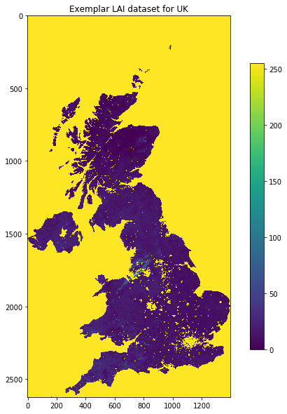
3.6.3.1 load an exemplar dataset
Since we want to match up datasets, we need to produce an example of the dataset we want to match up to.
We save the exemplar as a GeoTiff format file here.
from osgeo import gdal, gdalconst,osr
import numpy as np
from geog0111.process_timeseries import mosaic_and_clip

# set to True if you want to override
# the MODIS projection (see above)
use_6974 = False

'''
https://stackoverflow.com/questions/10454316/
how-to-project-and-resample-a-grid-to-match-another-grid-with-gdal-python
'''

# first get an exemplar LAI file, clipped to
# the required limits. We will use this to match
# the t2 dataset to
match_filename = mosaic_and_clip(tiles,1,year,ofolder='tmp',\
                    country_code=country_code,shpfile=shpfile,frmat='GTiff')

print(match_filename)

'''
Now get the projection, geotransform and dataset
size that we want to match to
'''
match_ds = gdal.Open(match_filename, gdalconst.GA_ReadOnly)
match_proj = match_ds.GetProjection()
match_geotrans = match_ds.GetGeoTransform()
wide = match_ds.RasterXSize
high = match_ds.RasterYSize

print('\nProjection from file:')
print(match_proj,'\n')

'''
set Projection 6974 from SR-OR
by setting use_6974 = True
'''
if use_6974:
    print('\nProjection 6974 from SR-ORG:')
    modis_wkt = 'data/modis_6974.wkt'
    match_proj = open(modis_wkt,'r').readline()
    match_ds.SetProjection(match_proj)
    print(match_proj,'\n')

'''
Visualise
'''
plt.figure(figsize=(10,10))
plt.title(f'Exemplar LAI dataset for {country_code}')
plt.imshow(match_ds.ReadAsArray())
plt.colorbar(shrink=0.75)
# close the file -- we dont need it any more
del match_ds
tmp/Lai_500m_2017_001_UK.tif

Projection from file:
PROJCS["unnamed",GEOGCS["Unknown datum based upon the custom spheroid",DATUM["Not_specified_based_on_custom_spheroid",SPHEROID["Custom spheroid",6371007.181,0]],PRIMEM["Greenwich",0],UNIT["degree",0.0174532925199433]],PROJECTION["Sinusoidal"],PARAMETER["longitude_of_center",0],PARAMETER["false_easting",0],PARAMETER["false_northing",0],UNIT["metre",1,AUTHORITY["EPSG","9001"]]]
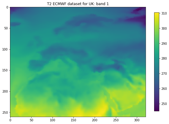
3.6.3.2 get information from source file
Now, we pull the information we need from the source file (the netcdf format t2 dataset).
We need to know:
- the data type
- the number of bands (time samples in this case)
- the geotransform of the dataset (the fact that it’s 0.25 degree resolution over Europe)
and access these from the source dataset.
from osgeo import gdal, gdalconst,osr
import numpy as np

# set up conditions
src_filename = f'data/europe_data_{year}.nc'
'''
access information from source
'''
src_dataname = 'NETCDF:"'+src_filename+'":t2m'
src     = gdal.Open(src_filename, gdalconst.GA_ReadOnly)

'''
Get geotrans, data type and number of bands
from source dataset
'''
band1 = src.GetRasterBand(1)
src_proj = src.GetProjection()
src_geotrans = src.GetGeoTransform()
nbands = src.RasterCount
src_format = band1.DataType
nx = band1.XSize
ny = band1.YSize

print('Information found')
print('GeoTransform:   ',src_geotrans)
print('Projection:     ',src_proj)
print('number of bands:',nbands)
print('format:         ',src_format)
print('nx,ny:          ',nx,ny)

# read data
t2m = band1.ReadAsArray()
plt.figure(figsize=(10,10))
ax = plt.subplot ( 1, 1, 1)
ax.set_title(f'T2 ECMWF dataset for {country_code}: band 1')

im = plt.imshow(t2m)
_ = plt.colorbar(im,shrink=0.6)
Information found
GeoTransform:    (-20.125, 0.25, 0.0, 75.125, 0.0, -0.25)
Projection:      GEOGCS["Coordinate System imported from GRIB file",DATUM["unknown",SPHEROID["Sphere",6371200,0]],PRIMEM["Greenwich",0],UNIT["degree",0.0174532925199433]]
number of bands: 365
format:          6
nx,ny:           321 261
3.6.3.4 reprojection
Now, set up a blank gdal dataset (in memory) with the size, data type, projection etc. that we want, the reproject the temperature dataset into this.
The processing may take some time if the LAI dataset is large (e.g. France).
The result will be of the same size, projection etc as the cropped LAI dataset.
dst_filename = src_filename.replace('.nc',f'_{country_code}.tif')
force = False


if (not Path(dst_filename).exists()) or force:

    dst = gdal.GetDriverByName('MEM').Create('', wide, high, nbands, src_format)

    dst.SetGeoTransform( match_geotrans )
    dst.SetProjection( match_proj)

    print('Information found')
    print('wide:      ',wide)
    print('high:      ',high)
    print('geotrans:  ',match_geotrans)
    print('projection:',match_proj)

    # Do the work: reproject the dataset
    # This will take a few minutes, depending on dataset size
    _ = gdal.ReprojectImage(src, dst, src_proj, match_proj, gdalconst.GRA_Bilinear)
xOrigin = match_geotrans[0]
yOrigin = match_geotrans[3]
pixelWidth = match_geotrans[1]
pixelHeight = match_geotrans[5]

extent = (xOrigin,xOrigin+pixelWidth*wide,\
         yOrigin+pixelHeight*(high),yOrigin+pixelHeight)

print(extent)

if (not Path(dst_filename).exists()) or force:


    '''
    Visualise: takes some time to plot
               due to reprojections
    '''
    t2m = dst.GetRasterBand(1).ReadAsArray()
    match_ds = gdal.Open(match_filename, gdalconst.GA_ReadOnly).ReadAsArray()

    # visualise
    plt.figure(figsize=(15,10))
    ax = plt.subplot ( 1, 2, 1 ,projection=ccrs.Sinusoidal.MODIS)
    ax.coastlines('10m')
    ax.set_title(f'T2m ECMWF dataset for {country_code}: band 1')
    im = ax.imshow(t2m[::-1],extent=extent)
    plt.colorbar(im,shrink=0.75)


    ax = plt.subplot ( 1, 2, 2 ,projection=ccrs.Sinusoidal.MODIS)
    ax.coastlines('10m')
    ax.set_title(f'MODIS LAI {country_code}')
    im = plt.imshow(match_ds,extent=extent)
    _ = plt.colorbar(im,shrink=0.75)
(-528121.3116353625, 118541.0173548233, 5549929.5167459585, 6765137.823590214)
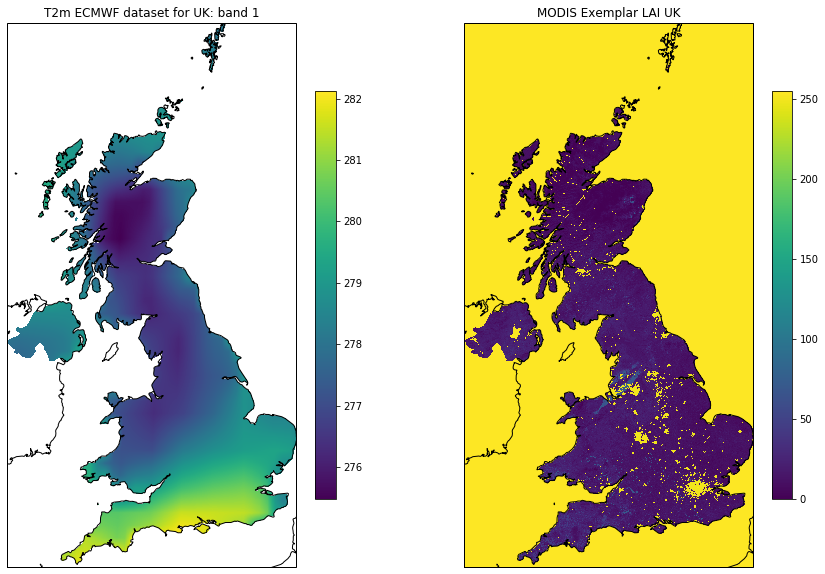
3.6.3.5 crop
Finally, we crop the temperature dataset using gdal.Warp() and save
it to a (GeoTiff) file:
 # Output / destination
dst_filename = src_filename.replace('.nc',f'_{country_code}.tif')
force = False


if (not Path(dst_filename).exists()) or force:
    '''
    Only run this if file doesnt exist
    '''
    frmat = 'GTiff'
    g = gdal.Warp(dst_filename,
                dst,
                format=frmat,
                dstNodata=-300,
                cutlineDSName=shpfile,
                cutlineWhere=f"FIPS='{country_code:s}'",
                cropToCutline=True)
    del dst # Flush
    del g
# visualise
print(dst_filename)
t2m = gdal.Open(dst_filename, gdalconst.GA_ReadOnly)
t2m = t2m.GetRasterBand(1).ReadAsArray()
t2m[t2m==-300] = np.nan
match_ds = gdal.Open(match_filename, gdalconst.GA_ReadOnly).ReadAsArray()

# visualise
plt.figure(figsize=(15,10))
ax = plt.subplot ( 1, 2, 1 ,projection=ccrs.Sinusoidal.MODIS)
ax.coastlines('10m')
ax.set_title(f'T2m ECMWF dataset for {country_code}: band 1')
im = ax.imshow(t2m[::-1],extent=extent)
plt.colorbar(im,shrink=0.75)

ax = plt.subplot ( 1, 2, 2 ,projection=ccrs.Sinusoidal.MODIS)
ax.coastlines('10m')
ax.set_title(f'MODIS Exemplar LAI {country_code}')
im = plt.imshow(match_ds,extent=extent)
_ = plt.colorbar(im,shrink=0.75)
data/europe_data_2017_UK.tif
Now let’s look at the time information in the metadata:
meta = gdal.Open(src_filename).GetMetadata()

print(meta['time#units'])
hours since 1900-01-01 00:00:00.0
The time information is in hours since 1900-01-01 00:00:00.0. This
is not such a convenient unit for plotting, so we can use datetime
to fix that:
timer = meta['NETCDF_DIM_time_VALUES']
print(timer[:100])
{1025628,1025652,1025676,1025700,1025724,1025748,1025772,1025796,1025820,1025844,1025868,1025892,102
# split the string into integers
timer = [int(i) for i in meta['NETCDF_DIM_time_VALUES'][1:-1].split(',')]

print (timer[:20])
[1025628, 1025652, 1025676, 1025700, 1025724, 1025748, 1025772, 1025796, 1025820, 1025844, 1025868, 1025892, 1025916, 1025940, 1025964, 1025988, 1026012, 1026036, 1026060, 1026084]
# split the string into integers
# convert to days
timer = [float(i)/24. for i in meta['NETCDF_DIM_time_VALUES'][1:-1].split(',')]

print (timer[:20])
[42734.5, 42735.5, 42736.5, 42737.5, 42738.5, 42739.5, 42740.5, 42741.5, 42742.5, 42743.5, 42744.5, 42745.5, 42746.5, 42747.5, 42748.5, 42749.5, 42750.5, 42751.5, 42752.5, 42753.5]
from datetime import datetime,timedelta

# add base date
# split the string into integers
# convert to days
timer = [(datetime(1900,1,1) + timedelta(days=float(i)/24.)) \
         for i in meta['NETCDF_DIM_time_VALUES'][1:-1].split(',')]

print (timer[:20])
[datetime.datetime(2017, 1, 1, 12, 0), datetime.datetime(2017, 1, 2, 12, 0), datetime.datetime(2017, 1, 3, 12, 0), datetime.datetime(2017, 1, 4, 12, 0), datetime.datetime(2017, 1, 5, 12, 0), datetime.datetime(2017, 1, 6, 12, 0), datetime.datetime(2017, 1, 7, 12, 0), datetime.datetime(2017, 1, 8, 12, 0), datetime.datetime(2017, 1, 9, 12, 0), datetime.datetime(2017, 1, 10, 12, 0), datetime.datetime(2017, 1, 11, 12, 0), datetime.datetime(2017, 1, 12, 12, 0), datetime.datetime(2017, 1, 13, 12, 0), datetime.datetime(2017, 1, 14, 12, 0), datetime.datetime(2017, 1, 15, 12, 0), datetime.datetime(2017, 1, 16, 12, 0), datetime.datetime(2017, 1, 17, 12, 0), datetime.datetime(2017, 1, 18, 12, 0), datetime.datetime(2017, 1, 19, 12, 0), datetime.datetime(2017, 1, 20, 12, 0)]
3.6.3.6 Putting this together
We can now put these codes together to make a function
match_netcdf_to_data():
from osgeo import gdal, gdalconst,osr
import numpy as np
from geog0111.process_timeseries import mosaic_and_clip
from datetime import datetime

def match_netcdf_to_data(src_filename,match_filename,dst_filename,year,\
                         country_code=None,shpfile=None,force=False,\
                         nodata=-300,frmat='GTiff',verbose=False):

    '''
    see :
    https://stackoverflow.com/questions/10454316/
    how-to-project-and-resample-a-grid-to-match-another-grid-with-gdal-python
    '''

    '''
    Get the projection, geotransform and dataset
    size that we want to match to
    '''
    if verbose: print(f'getting info from match file {match_filename}')
    match_ds = gdal.Open(match_filename, gdalconst.GA_ReadOnly)

    match_proj = match_ds.GetProjection()
    match_geotrans = match_ds.GetGeoTransform()
    wide = match_ds.RasterXSize
    high = match_ds.RasterYSize
    # close the file -- we dont need it any more
    del match_ds

    '''
    access information from source
    '''
    if verbose: print(f'getting info from source netcdf file {src_filename}')
    try:
        src_dataname = 'NETCDF:"'+src_filename+'":t2m'
        src = gdal.Open(src_dataname, gdalconst.GA_ReadOnly)
    except:
        if verbose: print('failed')
        return(None)

    # get meta data
    meta = gdal.Open(src_filename, gdalconst.GA_ReadOnly).GetMetadata()

    extent = [match_geotrans[0],match_geotrans[0]+match_geotrans[1]*wide,\
              match_geotrans[3]+match_geotrans[5]*high,match_geotrans[3]]
    # get time info
    timer = np.array([(datetime(1900,1,1) + timedelta(days=float(i)/24.)) \
         for i in meta['NETCDF_DIM_time_VALUES'][1:-1].split(',')])

    if (not Path(dst_filename).exists()) or force:

        '''
        Get geotrans, proj, data type and number of bands
        from source dataset
        '''
        band1 = src.GetRasterBand(1)
        src_geotrans = src.GetGeoTransform()
        src_proj = src.GetProjection()

        nbands = src.RasterCount
        src_format = band1.DataType

        dst = gdal.GetDriverByName('MEM').Create(\
                                        '', wide, high, \
                                        nbands, src_format)
        dst.SetGeoTransform( match_geotrans )
        dst.SetProjection( match_proj)

        if verbose: print(f'reprojecting ...')
            # Output / destination
        _ = gdal.ReprojectImage(src, dst, \
                                    src_proj, \
                                    match_proj,\
                                    gdalconst.GRA_Bilinear )
        if verbose: print(f'cropping to {country_code:s} ...')
        done = gdal.Warp(dst_filename,
                        dst,
                        format=frmat,
                        dstNodata=nodata,
                        cutlineDSName=shpfile,
                        cutlineWhere=f"FIPS='{country_code:s}'",
                        cropToCutline=True)
        del dst

    return(timer,dst_filename,extent)
from osgeo import gdal, gdalconst,osr
import numpy as np
from geog0111.process_timeseries import mosaic_and_clip
from datetime import datetime,timedelta
from geog0111.match_netcdf_to_data import match_netcdf_to_data
from geog0111.geog_data import procure_dataset
from pathlib import Path

# set conditions

country_code = 'UK'
year = 2017
shpfile = "data/TM_WORLD_BORDERS-0.3.shp"
src_filename = f'data/europe_data_{year}.nc'
dst_filename = f'data/europe_data_{year}_{country_code}.tif'
t2_filename = f'data/europe_data_{year}_{country_code}.npz'
# read in the LAI data for given country code
tiles = []
for h in [17, 18]:
    for v in [3, 4]:
        tiles.append(f"h{h:02d}v{v:02d}")


#read LAI
fname = f'lai_data_{year}_{country_code}.npz'
ofile = Path('data')/fname
lai = np.load(ofile)

if not Path(t2_filename).exists():
    print(f'calculating dataset match in {t2_filename}')
    # first get an exemplar LAI file, clipped to
    # the required limits. We will use this to match
    # the t2 dataset to
    match_filename = mosaic_and_clip(tiles,1,year,\
                        country_code=country_code,\
                        shpfile=shpfile,frmat='GTiff')
    '''
    Match the datasets using the function
    we have developed
    '''
    meta = gdal.Open(src_filename, gdalconst.GA_ReadOnly).GetMetadata()

    timer,dst_filename,extent = match_netcdf_to_data(\
                                    src_filename,match_filename,\
                                    dst_filename,year,\
                                    country_code=country_code,\
                                    shpfile=shpfile,\
                                    nodata=-300,frmat='GTiff',\
                                    verbose=True)

    # read and interpret the t2 data and flip
    temp2 = gdal.Open(dst_filename).ReadAsArray()[:,::-1]
    temp2[temp2==-300] = np.nan
    temp2 -= 273.15
    # save these
    print(f'saving data to {t2_filename}')
    np.savez_compressed(t2_filename,timer=timer,temp2=temp2,extent=extent)

else:
    print(f'dataset in {t2_filename} exists')

print('done')
t2data = np.load(t2_filename)
timer,temp2,extent = t2data['timer'],t2data['temp2'],t2data['extent']
calculating dataset match in data/europe_data_2017_UK.npz
getting info from match file data/Lai_500m_2017_001_UK.tif
getting info from source netcdf file data/europe_data_2017.nc
saving data to data/europe_data_2017_UK.npz
done
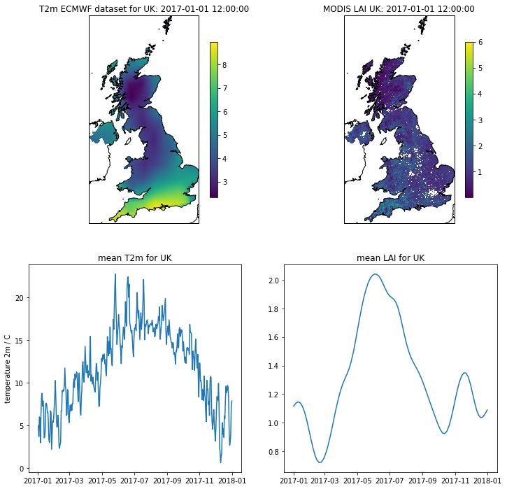
# visualise the interpolated dataset
import matplotlib.pylab as plt
import cartopy.crs as ccrs
%matplotlib inline

plt.figure(figsize=(12,12))
ax = plt.subplot ( 2, 2, 1 ,projection=ccrs.Sinusoidal.MODIS)
ax.coastlines('10m')
ax.set_title(f'T2m ECMWF dataset for {country_code}: {str(timer[0])}')
im = ax.imshow(temp2[0],extent=extent)
plt.colorbar(im,shrink=0.75)

ax = plt.subplot ( 2, 2, 2 ,projection=ccrs.Sinusoidal.MODIS)
ax.coastlines('10m')
ax.set_title(f'MODIS LAI {country_code}: {str(timer[0])}')
im = plt.imshow(interpolated_lai[:,:,0],vmax=6,extent=extent)
_ = plt.colorbar(im,shrink=0.75)

plt.subplot ( 2, 2, 3 )
plt.title(f'mean T2m for {country_code}')
plt.plot(timer,np.nanmean(temp2,axis=(1,2)))
plt.ylabel('temperature 2m / C')
plt.subplot ( 2, 2, 4 )
plt.title(f'mean LAI for {country_code}')
mean = np.nanmean(interpolated_lai,axis=(0,1))
plt.plot(timer[::4],mean)
[<matplotlib.lines.Line2D at 0x11dc20b38>]
3.6.6 Summary
In this section, we have learned about projections, and have reconciled two datasets that were originally in different projections. NThey also were defined with geoids with different Earth radius assumptions.
These issues are typical when dealing with geospatial data.
This part of the notes is non compulsory, as the codes and ideas are quite complicated for people just begining to learn coding. We have included it here to allow students to revisit this later. It is also included because we want to develop some interesting datasets for modelling, so we need to deal with reconciling datasets from different providers in different projections.
In this section, we have developed the following datasets:
from geog0111.geog_data import procure_dataset
import numpy as np
from pathlib import Path

year = 2017
country_code = 'UK'
'''
LAI data
'''
# read in the LAI data for given country code
lai_filename = f'data/lai_data_{year}_{country_code}.npz'
# get the dataset in case its not here
procure_dataset(Path(lai_filename).name,verbose=False)

lai = np.load(lai_filename)
print(lai_filename,list(lai.keys()))

'''
T 2m data
'''
t2_filename = f'data/europe_data_{year}_{country_code}.npz'
# get the dataset in case its not here
procure_dataset(Path(t2_filename).name,verbose=False)
t2data = np.load(t2_filename)
print(t2_filename,list(t2data.keys()))
data/lai_data_2017_UK.npz ['dates', 'lai', 'weights', 'interpolated_lai']
data/europe_data_2017_UK.npz ['timer', 'temp2', 'extent']
import numpy as np
# a quick look at some stats to see if there are data there
# and they are sensible
lai = np.load(ofile)
print(np.array(lai['lai'][1000,700]),\
      np.array(lai['weights'][1000,700]))
# does it have the interpolated value?
if 'interpolated_lai' in list(lai.keys()):
    print(np.array(lai['interpolated_lai'][1000,700]))
[1.1 1.1 1.2 0.9 0.9 1.2 1.  0.8 1.4 0.3 0.  0.5 0.3 0.9 0.6 1.  0.7 0.5
 0.7 0.6 1.3 0.7 0.1 1.  1.  0.6 1.1 0.5 1.1 1.  1.1 1.1 1.1 0.  0.6 1.4
 1.3 1.6 1.7 1.7 1.1 0.3 1.3 1.7 1.5 1.2 0.5 0.6 1.6 3.1 0.3 2.  1.6 0.5
 2.6 2.5 0.4 0.4 0.4 0.4 0.4 1.1 1.7 0.5 1.5 1.4 0.1 1.4 1.  1.  0.3 1.1
 0.2 1.1 0.1 0.7 2.6 1.7 2.  1.4 1.4 0.3 0.4 0.7 1.1 1.1 0.8 0.8 0.9 1.2
 1.2 1.2] [0.38196601 0.38196601 0.38196601 0.38196601 0.38196601 0.38196601
 0.38196601 0.38196601 0.38196601 0.38196601 0.38196601 1.
 1.         1.         1.         1.         1.         1.
 1.         1.         1.         1.         1.         1.
 1.         1.         1.         1.         1.         1.
 1.         1.         1.         0.23606798 1.         1.
 1.         1.         1.         1.         0.23606798 0.23606798
 1.         1.         1.         1.         0.23606798 1.
 1.         1.         0.23606798 1.         1.         0.23606798
 1.         1.         0.23606798 0.23606798 0.23606798 0.23606798
 1.         1.         1.         1.         1.         1.
 1.         1.         1.         1.         1.         1.
 0.23606798 1.         1.         0.38196601 0.38196601 0.38196601
 0.38196601 0.38196601 0.38196601 0.38196601 0.38196601 0.38196601
 0.38196601 0.38196601 0.38196601 0.38196601 0.38196601 0.38196601
 0.38196601 0.38196601]
[1.08683704 1.07935938 1.06092468 1.03161555 0.99133678 0.93493706
 0.86317607 0.78136836 0.70352293 0.64487202 0.61266704 0.60678279
 0.61883651 0.63991235 0.66383767 0.68530728 0.7020839  0.71506691
 0.72433462 0.73247513 0.74002342 0.7487489  0.76081558 0.77753903
 0.79985155 0.82674875 0.8580399  0.89089931 0.92313233 0.95320821
 0.98065863 1.00873477 1.04290792 1.08866497 1.14943392 1.22080857
 1.2929335  1.35676154 1.4021202  1.42632177 1.43105239 1.41880135
 1.40112126 1.38702625 1.38535581 1.40496862 1.45132144 1.52190587
 1.6097794  1.70184005 1.78498301 1.84800873 1.88579434 1.89137779
 1.85216521 1.7573269  1.60194669 1.4068558  1.2226864  1.09378123
 1.03387865 1.01734516 1.02167784 1.02682062 1.02221966 1.00590369
 0.98109385 0.95002526 0.91607184 0.8832294  0.85542066 0.83730438
 0.83548611 0.85858254 0.90888448 0.98602178 1.07794995 1.15678679
 1.19786983 1.18422965 1.12426637 1.04138037 0.9671476  0.91852027
 0.90214004 0.90955621 0.93302657 0.96662729 1.00304032 1.03742083
 1.06445991 1.08219511]
Exercise 3.6.2 Extra Homework
Go carefully through these notes and make notes of the processes we have to go through to reconcile datasets such as these.
Learn what issues to look out for when coming across a new dataset, and
how to use Python code to deal with it. Try to stick to one geospatial
package as far as possible (gdal here) as you can make problems for
yourself by mixing them.
# do exercise here